1.2 — Budget Constraint
ECON 306 • Microeconomic Analysis • Spring 2023
Ryan Safner
Associate Professor of Economics
safner@hood.edu
ryansafner/microS23
microS23.classes.ryansafner.com
The Two Major Models of Economics as a “Science”
Optimization
Agents have objectives they value
Agents face constraints
Make tradeoffs to maximize objectives within constraints

Equilibrium
Agents compete with others over scarce resources
Agents adjust behaviors based on prices
Stable outcomes when adjustments stop

Rational Choice Theory
The Logic of Choice: Ends and Means
Each of us acts purposefully
We have ends, goals, desires, objectives
- Anything you value!
We use means in the world that we believe will achieve our ends
- “utility” when we consume services, or
- if scarce physical object: “economic good” or resource


The Logic of Choice: Purpose
Acting with purpose distinguishes humans from everything else in the universe
Artificial intelligence researchers face “the frame problem”
- Perception requires motivational goals to determine how to filter reality

Causal Inference I
Machine learning and artificial intelligence are “dumb”
- Data can never “speak for itself!”
With the right models and research designs, we can say “X causes Y” and quantify it!
Economists are in a unique position to make causal claims that mere statistics cannot

For more, see my blog post, and Pearl & MacKenzie (2018), The Book of Why
Causal Inference II
“First, the field of economics has spent decades developing a toolkit aimed at investigating empirical relationships, focusing on techniques to help understand which correlations speak to a causal relationship and which do not. This comes up all the time — does Uber Express Pool grow the full Uber user base, or simply draw in users from other Uber products? Should eBay advertise on Google, or does this simply syphon off people who would have come through organic search anyway? Are African-American Airbnb users rejected on the basis of their race? These are just a few of the countless questions that tech companies are grappling with, investing heavily in understanding the extent of a causal relationship.”
The Law of Demand
Perhaps the most fundamental economic “law” is the law of demand:
- inverse relationship between price and quantity consumed
- i.e. demand curves slope downwards
We investigate its source, and derive more useful properties
First, we will need to develop a more rigorous framework

Rational Choice Theory
How do people decide:
- which products to buy
- which activities to dedicate time to
- how much to save or invest
- how to plan for the future
Rational choice theory: assume that people optimize within constraints
A model of behavior we can extend to most scenarios

Rational Choice Theory: Beyond Consumers
Often called “Consumer Theory” in textbooks, but realize:
Everyone is “a consumer”
- "Goods and services" are anything that you value!
- Producers demand productive inputs
We are really modeling how individuals make choices in almost any context!

Consumption Bundles
Imagine a (very strange) supermarket sells x and y
Your choices: amounts of {x,y} to consume as a bundle

Consumption Bundles: Graphically
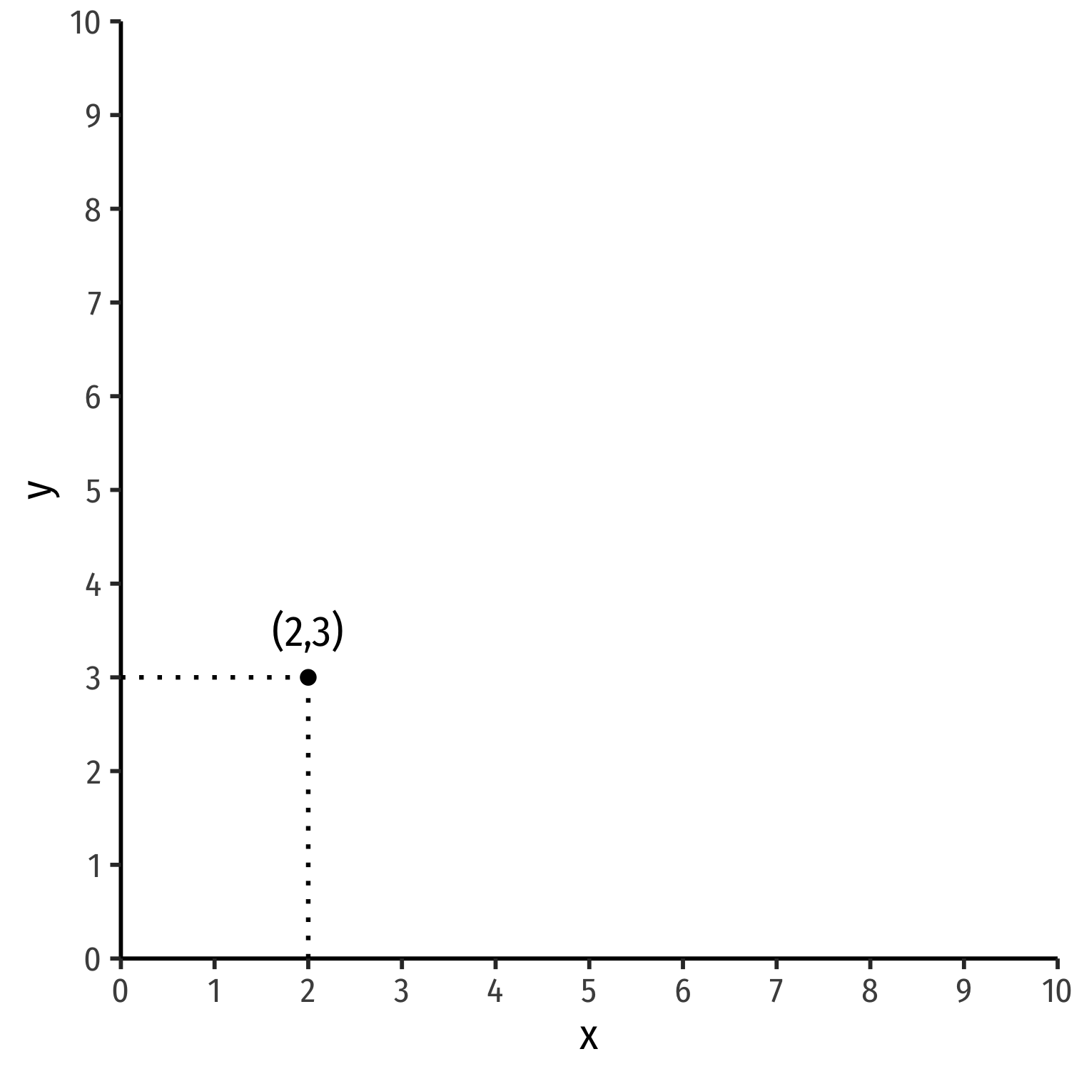
We can represent bundles graphically
We’ll stick with 2 goods (x,y) in 2-dimensions†
Example:
- x: 2 units
- y: 3 units
† See appendix in today's class page to extend to n goods!
The Budget Constraint
Affordability
If you had $100 to spend, what bundles of goods {x,y} would you buy?
Only those bundles that are affordable
Denote prices of each good as {px,py}
Let m be the amount of income a person has

Affordability
If you had $100 to spend, what bundles of goods {x,y} would you buy?
Only those bundles that are affordable
Denote prices of each good as {px,py}
Let m be the amount of income a person has
A bundle {x,y} is affordable at given prices {px,py} when:
pxx+pyy≤m

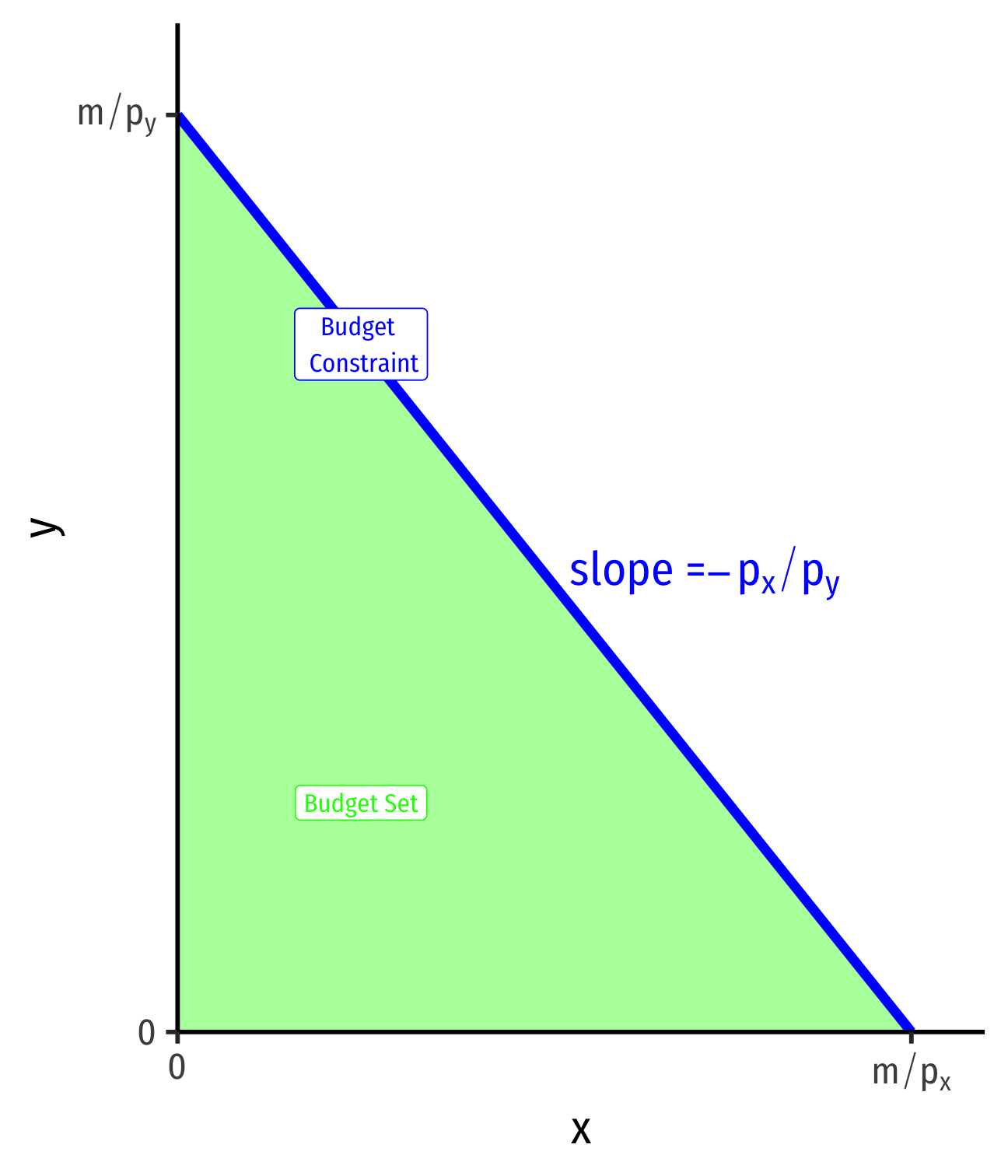
The Budget Set
- The set of all affordable bundles that a consumer can choose is called the budget set or choice set
pxx+pyy≤m

The Budget Set & the Budget Constraint
- The set of all affordable bundles that a consumer can choose is called the budget set or choice set
pxx+pyy≤m
- The budget constraint is the set of all bundles that spend all income m:†
pxx+pyy=m

† Note the difference (the in/equality): budget constraint is the subset of the budget set that spends all income.
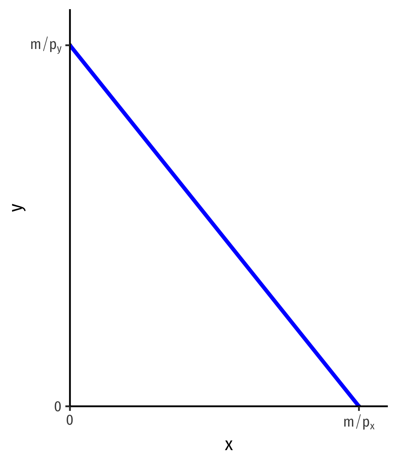
The Budget Constraint, Graphically
- For 2 goods, (x,y)
pxx+pyy=m
The Budget Constraint, Graphically
- For 2 goods, (x,y)
pxx+pyy=m
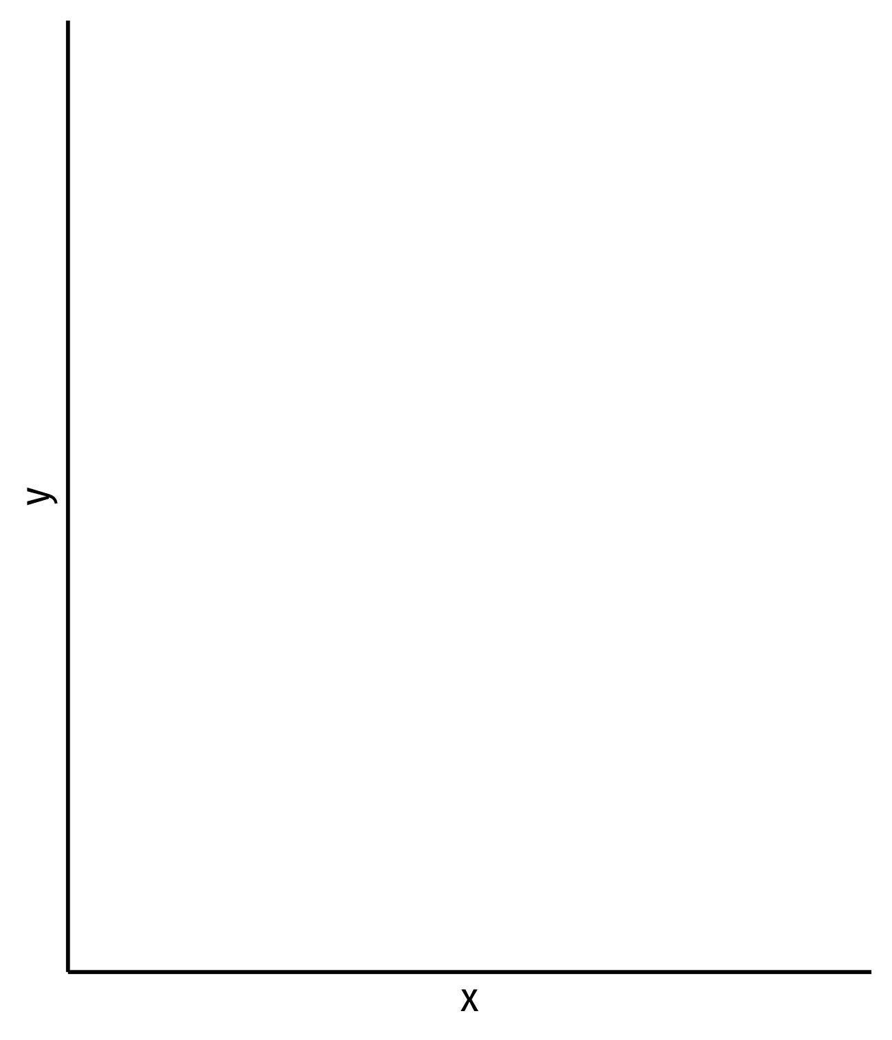
- Solve for y to graph
y=mpy−pxpyx
The Budget Constraint, Graphically
- For 2 goods, (x,y)
pxx+pyy=m
- Solve for y to graph
y=mpy−pxpyx
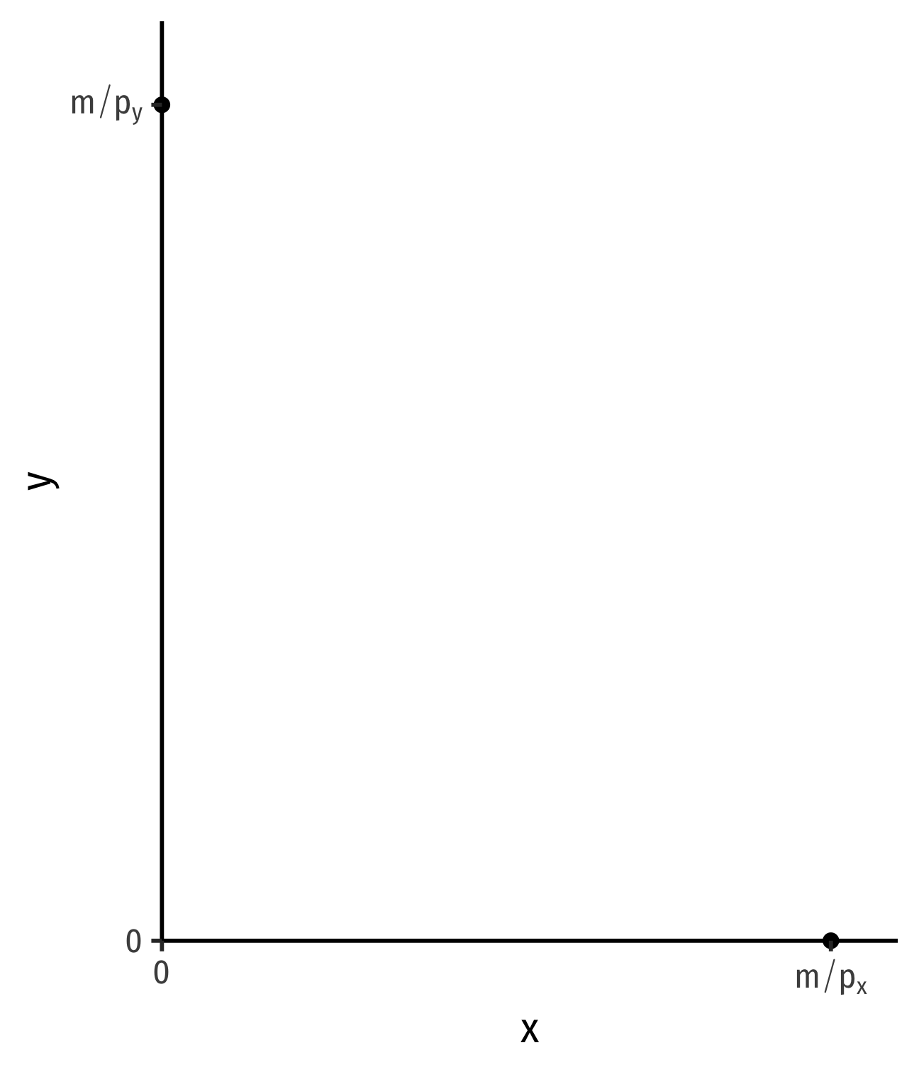
- y-intercept: mpy
- x-intercept: mpx
The Budget Constraint, Graphically
- For 2 goods, (x,y)
pxx+pyy=m
- Solve for y to graph
y=mpy−pxpyx
- y-intercept: mpy
- x-intercept: mpx
- slope: −pxpy
The Budget Constraint, Graphically
- For 2 goods, (x,y)
pxx+pyy=m
- Solve for y to graph
y=mpy−pxpyx
- y-intercept: mpy
- x-intercept: mpx
- slope: −pxpy
The Budget Constraint: Example
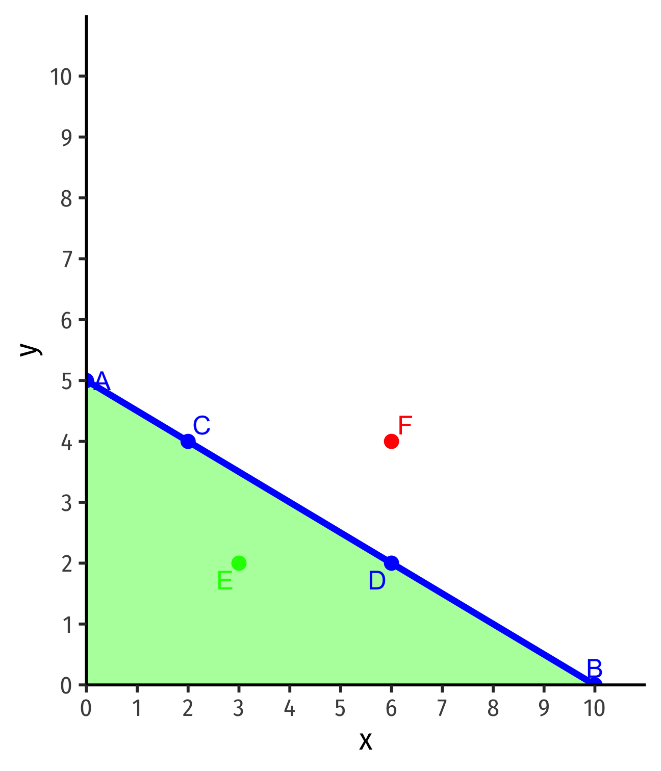
Example: Suppose you have an income of $50 to spend on lattes (l) and burritos (b). The price of lattes is $5 and the price of burritos is $10.
Let l be on the horizontal axis and b be on the vertical axis.
Write an equation for the budget constraint (in graphable form).
Graph the budget constraint.
Interpreting the Budget Constraint
- Points on the line spend all income
- A: $5(0x)+$10(5y)=$50
- B: $5(10x)+$10(0y)=$50
- C: $5(2x)+$10(4y)=$50
- D: $5(6x)+$10(2y)=$50

Interpreting the Budget Constraint
Points on the line spend all income
- A: $5(0x)+$10(5y)=$50
- B: $5(10x)+$10(0y)=$50
- C: $5(2x)+$10(4y)=$50
- D: $5(6x)+$10(2y)=$50
Points beneath line are affordable but don't use all income
- E: $5(3x)+$10(2y)=$35

Interpreting the Budget Constraint
Points on the line spend all income
- A: $5(0x)+$10(5y)=$50
- B: $5(10x)+$10(0y)=$50
- C: $5(2x)+$10(4y)=$50
- D: $5(6x)+$10(2y)=$50
Points beneath line are affordable but don't use all income
- E: $5(3x)+$10(2y)=$35
Points above line are unaffordable (now)
- F: $5(6x)+$10(4y)=$70
Opportunity Cost
Interpretting the Slope
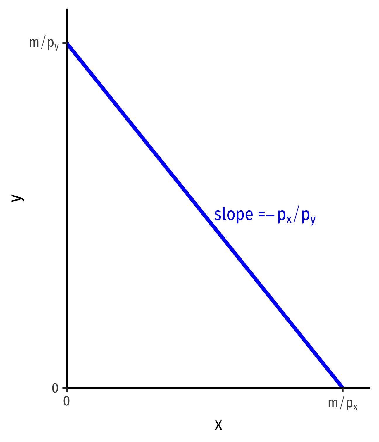
Slope: tradeoff between x and y at market prices
- Market “exchange rate”: pxpyy:1x
Relative price of x, or the opportunity cost of x:
Consuming 1 more unit of x requires giving up pxpy units of y

Opportunity Cost
Opportunity cost: value of next best foregone opportunity
Even though we use money for prices, when you consume x, you’re really giving up the opportunity to consume y!
The Parable of the Broken Window
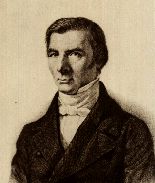
Frederic Bastiat
1801-1850
- That Which is Seen and That Which is Not Seen
The Parable of the Broken Window

Frederic Bastiat
1801-1850
That Which is Seen and That Which is Not Seen
“That which is seen”
- The broken window
- Resources diverted into glassmaking
The Parable of the Broken Window

Frederic Bastiat
1801-1850
That Which is Seen and That Which is Not Seen
“That which is seen”
- The broken window
- Resources diverted into glassmaking
“That which is not seen”
- Opportunity cost of fixing the window
- Resources diverted away from other opportunities
Applying the Parable of the Broken Window
- What does it mean to say that “spending money 'stimulates' the economy”?

Applying the Parable of the Broken Window
What does it mean to say that “spending money 'stimulates' the economy”?
Scarce resources used in one industry can not be used in other industries
Every (visible) decision to spend on X yields more X, and destroys an (invisible) opportunity to spend on Y

Could It Be Opportunity Cost (of Skilled Labor)?
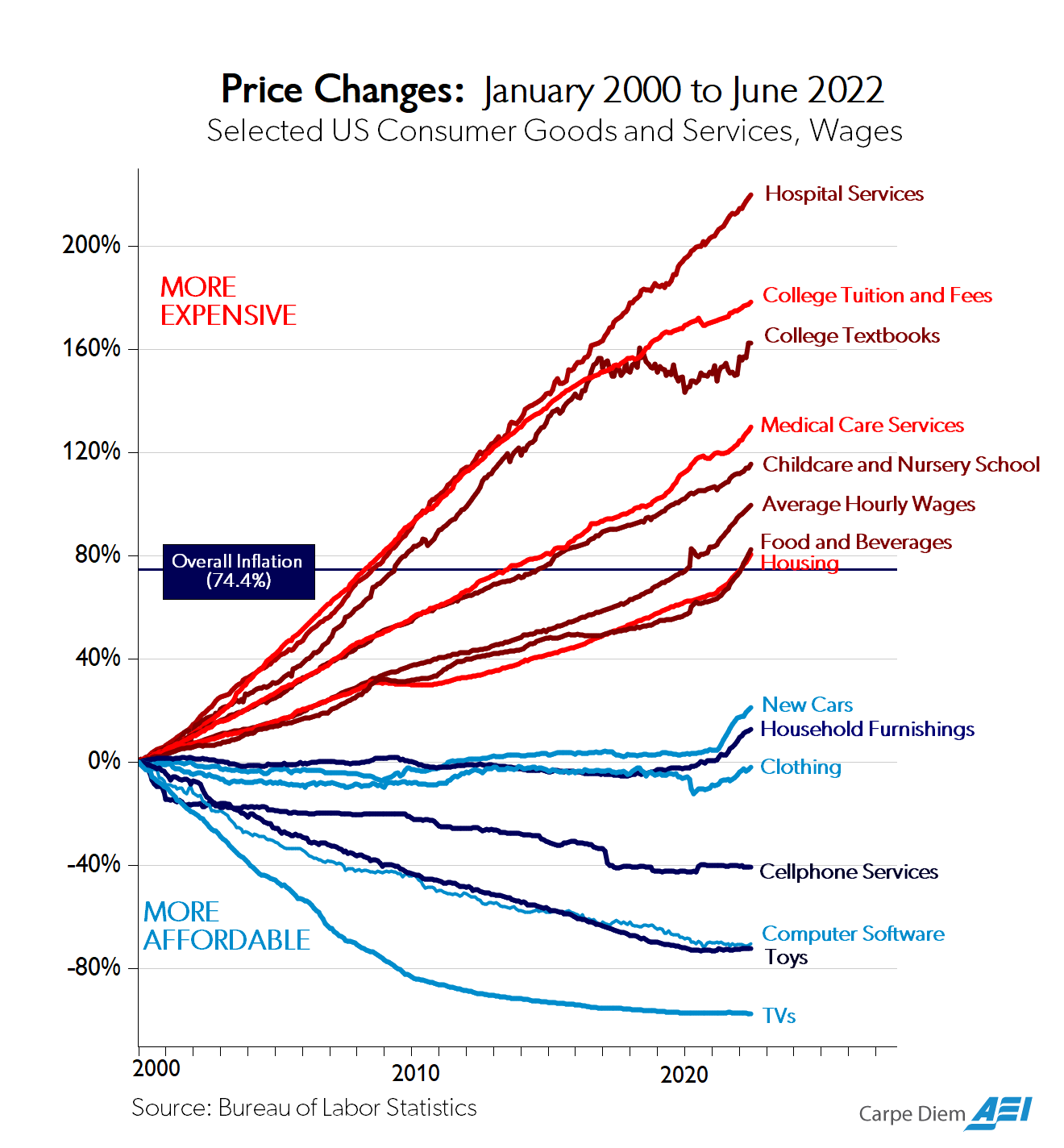
Source: Perry, Mark, 2022, “Chart of the Day...Or Century?” American Enterprise Institute
Could It Be Opportunity Cost (of Skilled Labor)?

“The Baumol effect is easy to explain but difficult to grasp. In 1826, when Beethoven’s String Quartet No. 14 was first played, it took four people 40 minutes to produce a performance. In 2010, it still took four people 40 minutes to produce a performance. Stated differently, in the nearly 200 years between 1826 and 2010, there was no growth in string quartet labor productivity. In 1826 it took 2.66 labor hours to produce one unit of output, and it took 2.66 labor hours to produce one unit of output in 2010.”
Sources: Helland, Eric and Alexander Tabarrok, 2019, “Why Are The Prices So Damn High?” Mercatus Center
Good summaries on Marginal Revolution
Could It Be Opportunity Cost (of Skilled Labor)?

“Fortunately, most other sectors of the economy have experienced substantial growth in labor productivity since 1826...In 1826 the average hourly wage for a production worker was $1.14. In 2010 the average hourly wage for a production worker was $26.44, approximately 23 times higher in real (inflation-adjusted) terms. Growth in average labor productivity has a surprising implication: it makes the output of slow productivity-growth sectors (relatively) more expensive. In 1826, the average wage of $1.14 meant that the 2.66 hours needed to produce a performance of Beethoven’s String Quartet No. 14 had an opportunity cost of just $3.02. At a wage of $26.44, the 2.66 hours of labor in music production had an opportunity cost of $70.33. Thus, in 2010 it was 23 times...more expensive to produce a performance of Beethoven’s String Quartet No. 14 than in 1826.”
Sources: Helland, Eric and Alexander Tabarrok, 2019, “Why Are The Prices So Damn High?” Mercatus Center
Good summaries on Marginal Revolution
Could It Be Opportunity Cost (of Skilled Labor)?

“In other words, one had to give up more other goods and services to produce a music performance in 2010 than one did in 1826. Why? Simply because in 2010, society was better at producing other goods and services than in 1826.”
Sources: Helland, Eric and Alexander Tabarrok, 2019, “Why Are The Prices So Damn High?” Mercatus Center
Good summaries on Marginal Revolution
Could It Be Opportunity Cost (of Skilled Labor)?

“The 23 times increase in the relative price of the string quartet is the driving force of Baumol’s cost disease. The focus on relative prices tells us that the cost disease is misnamed. The cost disease is not a disease but a blessing. To be sure, it would be better if productivity increased in all industries, but that is just to say that more is better. There is nothing negative about productivity growth, even if it is unbalanced.”
Sources: Helland, Eric and Alexander Tabarrok, 2019, “Why Are The Prices So Damn High?” Mercatus Center
Good summaries on Marginal Revolution
Changes in Market Conditions
Changes in Market Conditions
m=pxx+pyyy=mpy−pxpyx
Budget constraint is a function of specific parameters
- m: income
- px,py: market prices
Economic analysis: how changes in constraints affect people's choices
- “incentives”

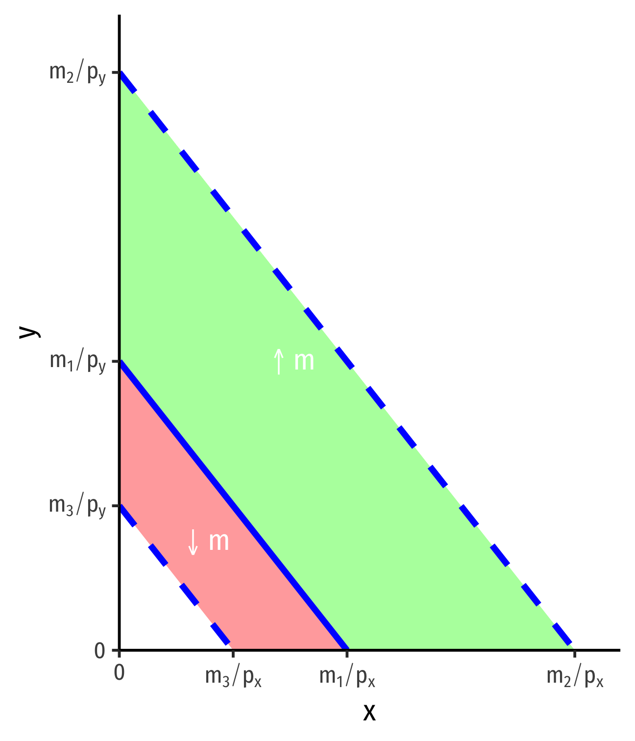
Changes in Income, m
- Changes in income shift the budget constraint
Example:
- Income increases m1→m2
- Income decreases m1→m3
Slope unchanged (no change in prices!)
Gain/loss of affordable bundles
Changes in Income, m: Example
Example: Continuing the lattes and burritos example, (income is $50, lattes are $5, burritos are $10), suppose your income doubles to $100.
Find the equation of the new budget constraint (in graphable form).
Graph the new budget constraint.
Changes in Relative Prices, px or py
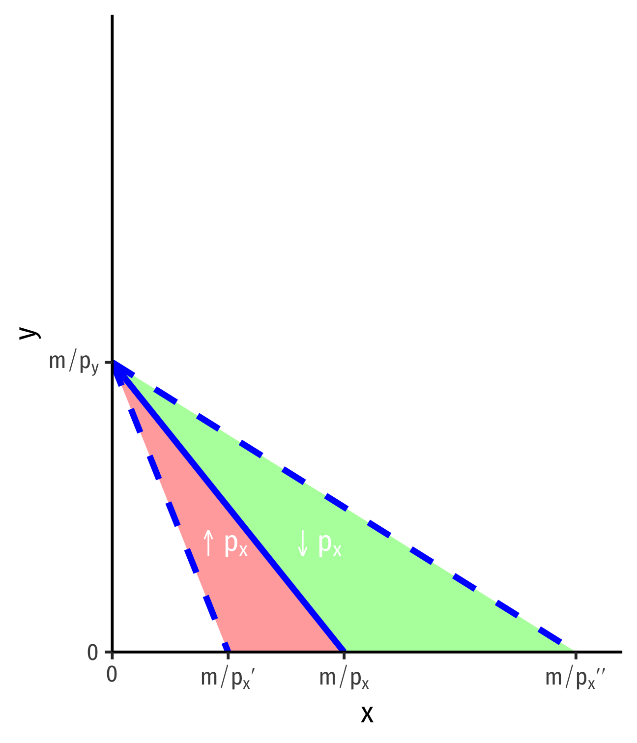
- Change in relative prices rotate the budget constraint
Example:
- Price of x increases px→p′x
- Price of x decreases px→p′′x
Change in slope: −p′xpy, −p′′xpy
Gain/loss of affordable bundles
Changes in Relative Prices, px or py
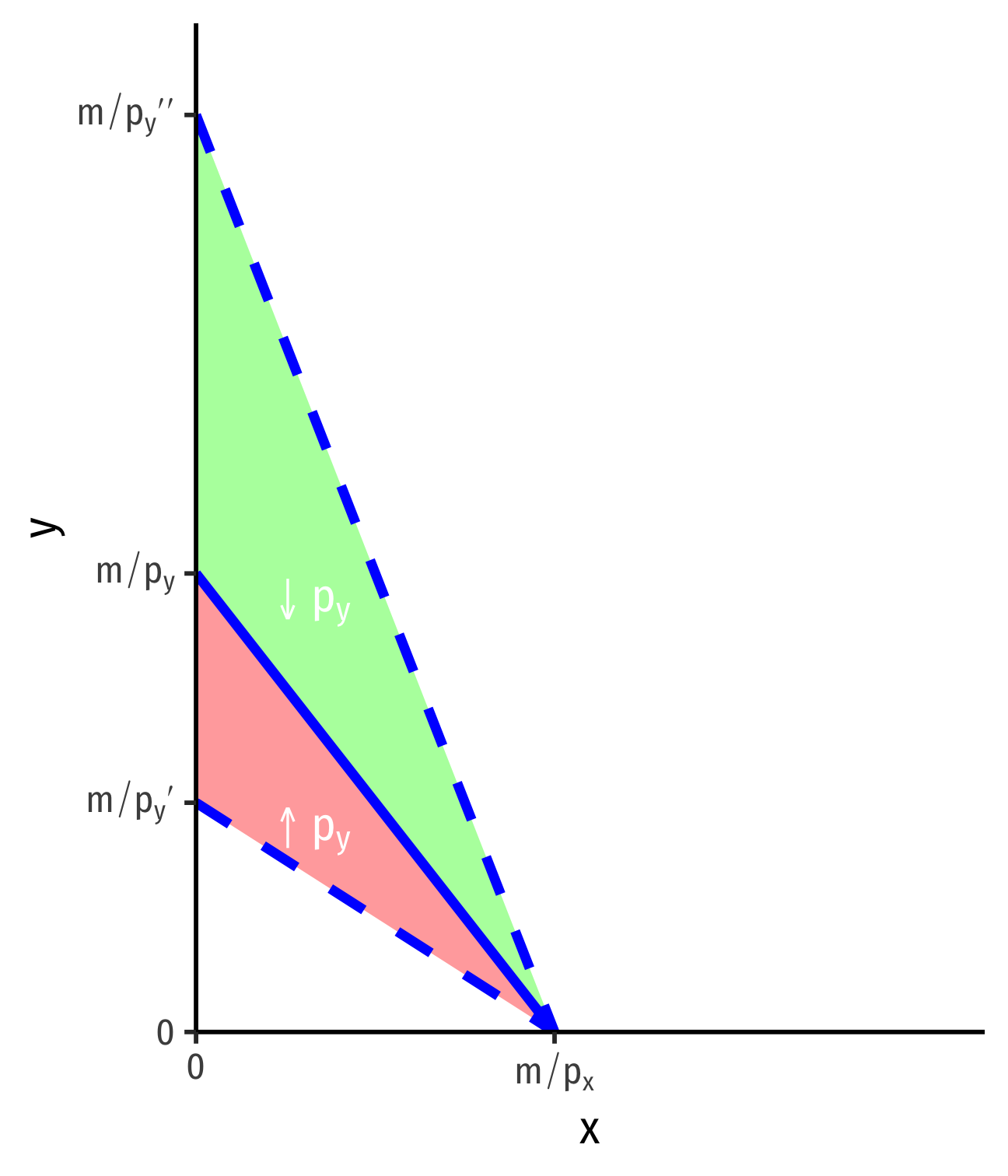
- Change in relative prices rotate the budget constraint
Example:
- Price of y increases py→p′y
- Price of y decreases py→p′′y
Change in slope: −pxp′y, −pxp′′y
Gain/loss of affordable bundles
Economics is About (Changes in) Relative Prices
Economic analysis is about (changes in) relative prices
Budget constraint slope (opportunity cost of x) is −pxpy
Only “real” changes in relative prices (from changes in market conditions) change consumer constraints (and alter behavior)
i.e. not “the price of x,” its about “the price of x relative to the price of y”!

Economics is About (Changes in) Relative Prices
- “Nominal” prices are often meaningless!
- Need to make comparisons between prices of different goods
Example: Imagine yourself in a strange country. All you know is that the price of bread, in local currency, is “6”...

Changes in Relative Prices: Example
Example: Continuing the lattes and burritos example (income is $50, lattes are $5, burritos are $10).
Suppose the price of lattes doubles from $5 to $10. Find the equation of the new budget constraint and graph it.
Return to the original price of lattes ($5) and suppose the price of burritos falls from $10 to $5. Find the equation of the new budget constraint and graph it.
Budget Constraint and the Law of Demand
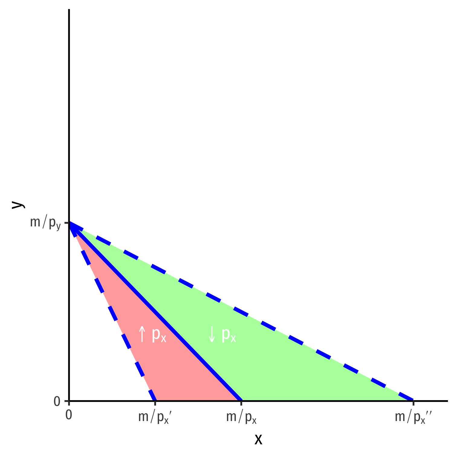
Recall the law of demand
We can derive it right off the budget constraint!
- As ↑px, person can consume less x
- As ↓px, person can consume more x
Notice I have made no assumptions about rationality, preferences, utility, etc to get this!
Markets Do Not Require Individual Rationality
A lot of griping about "rationality" and whether people are truly "rational"
- Behavioral economics, for example
The law of demand does not require rational people! (utility-maximizers, etc)
- or markets, for that matter, it's the direct result of scarcity
This is important: markets don't require rational people, they make people rational!

