1.7 — Price Elasticity

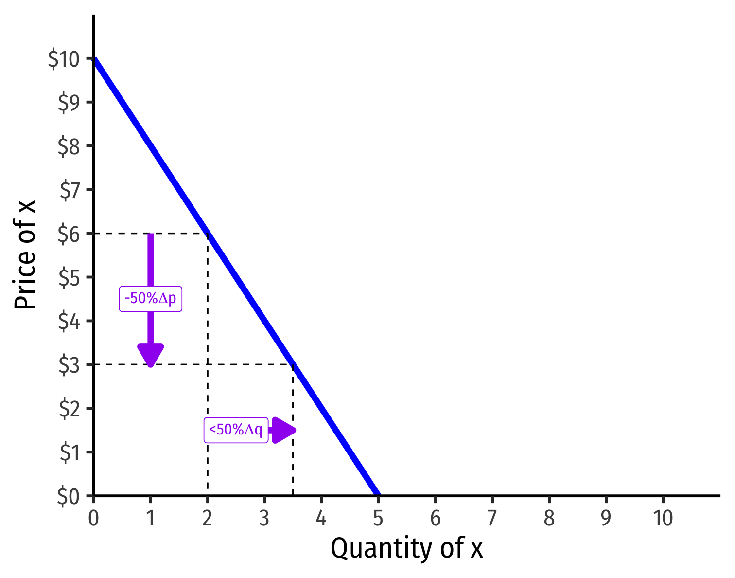
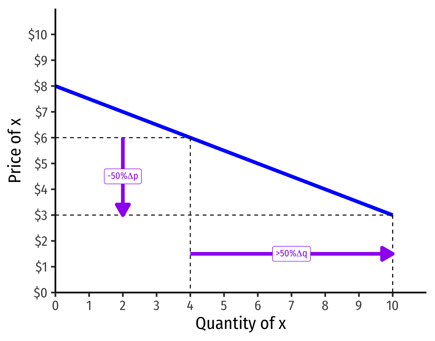
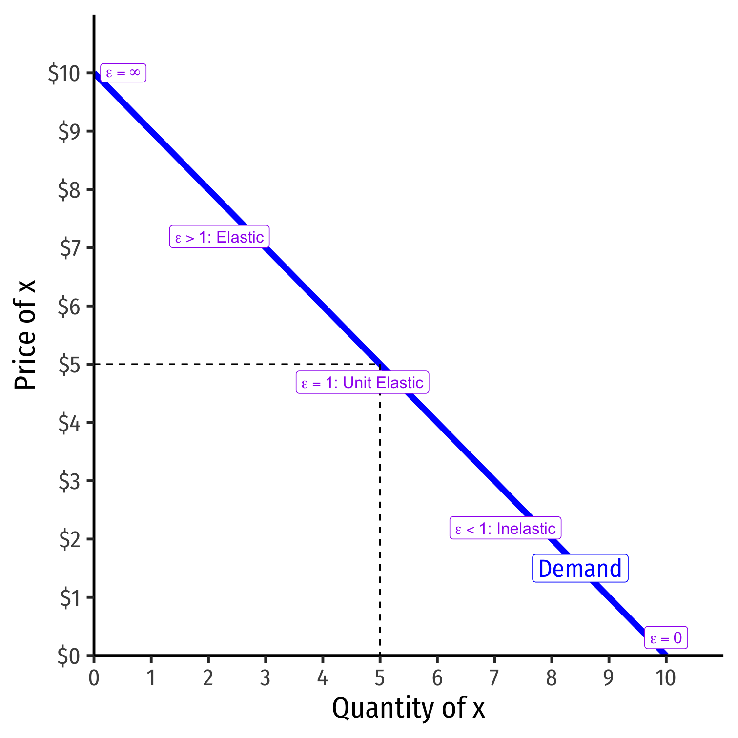
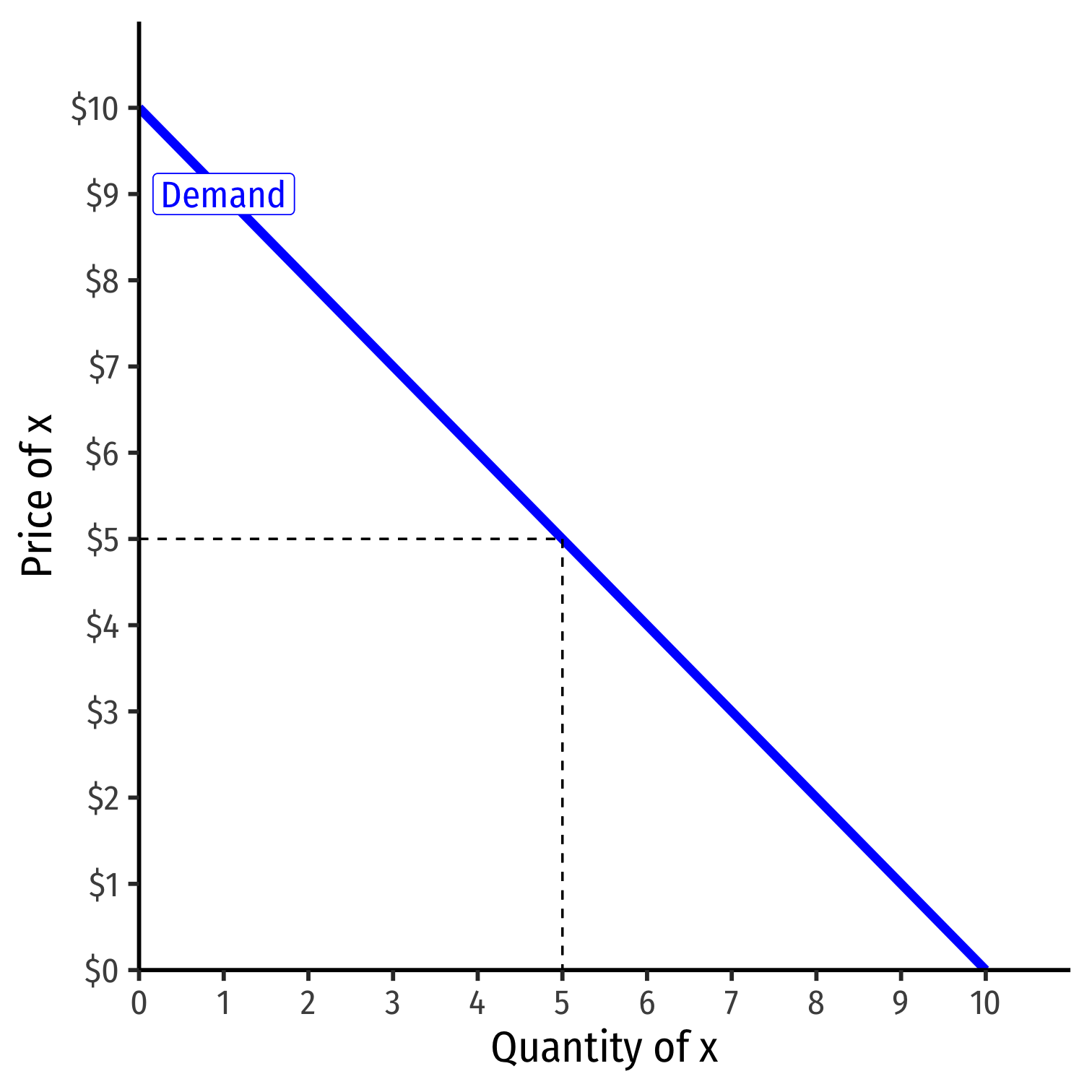
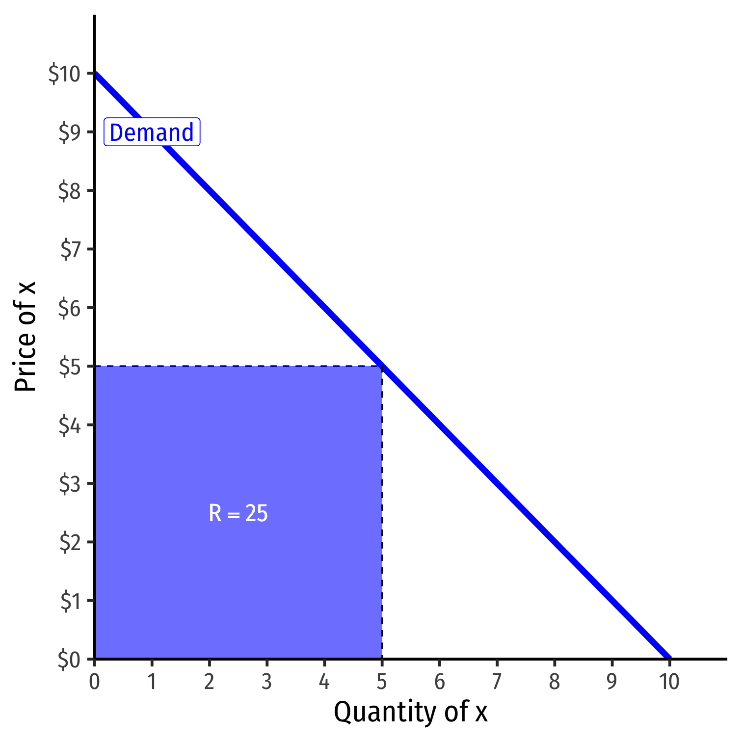
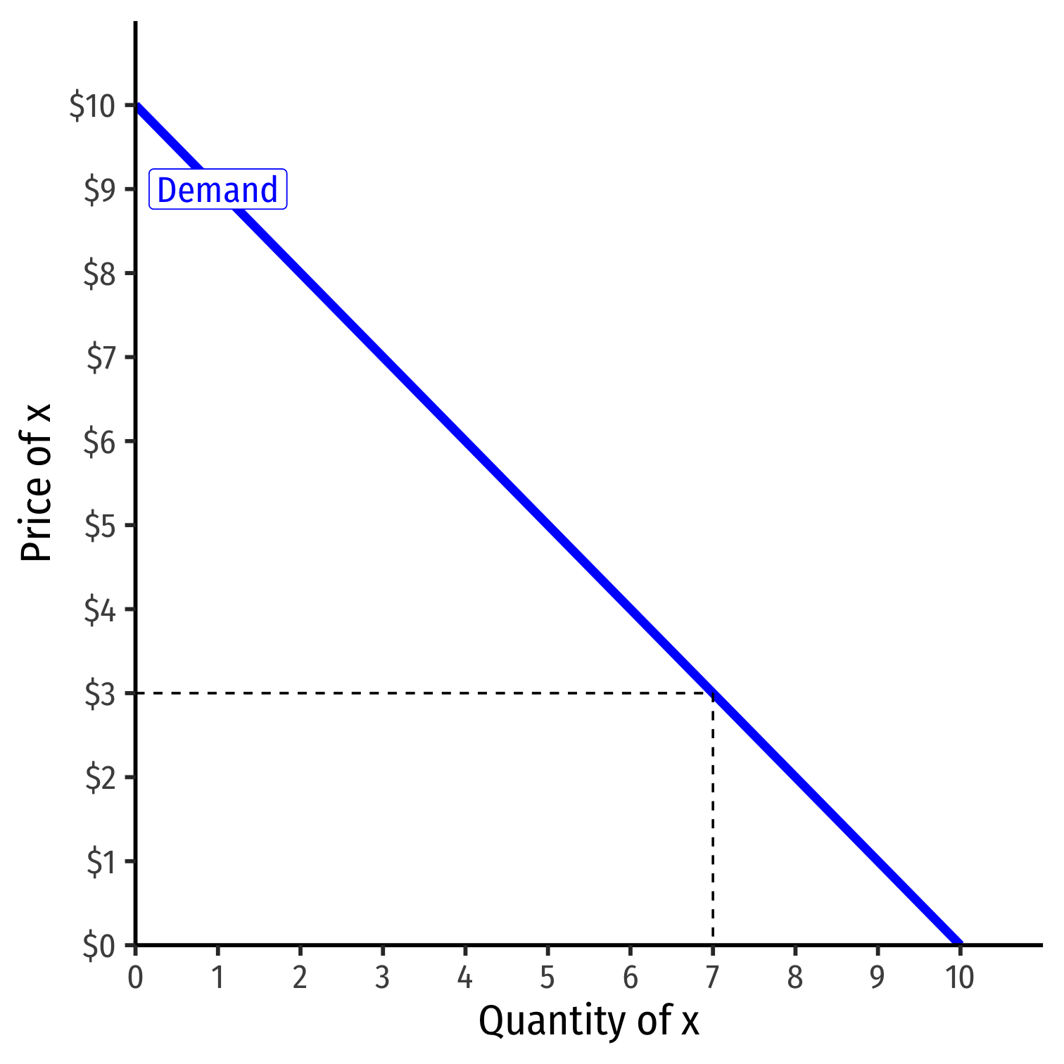
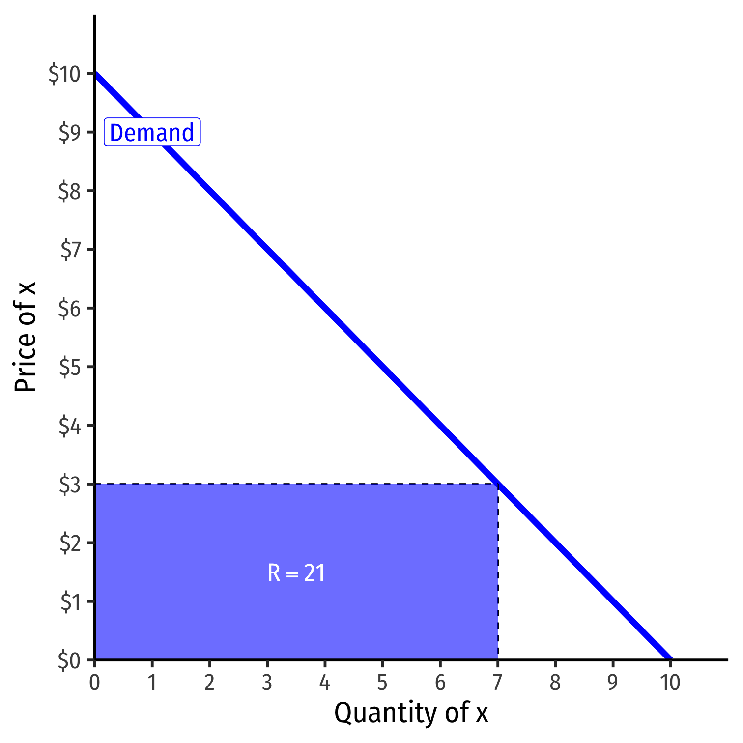
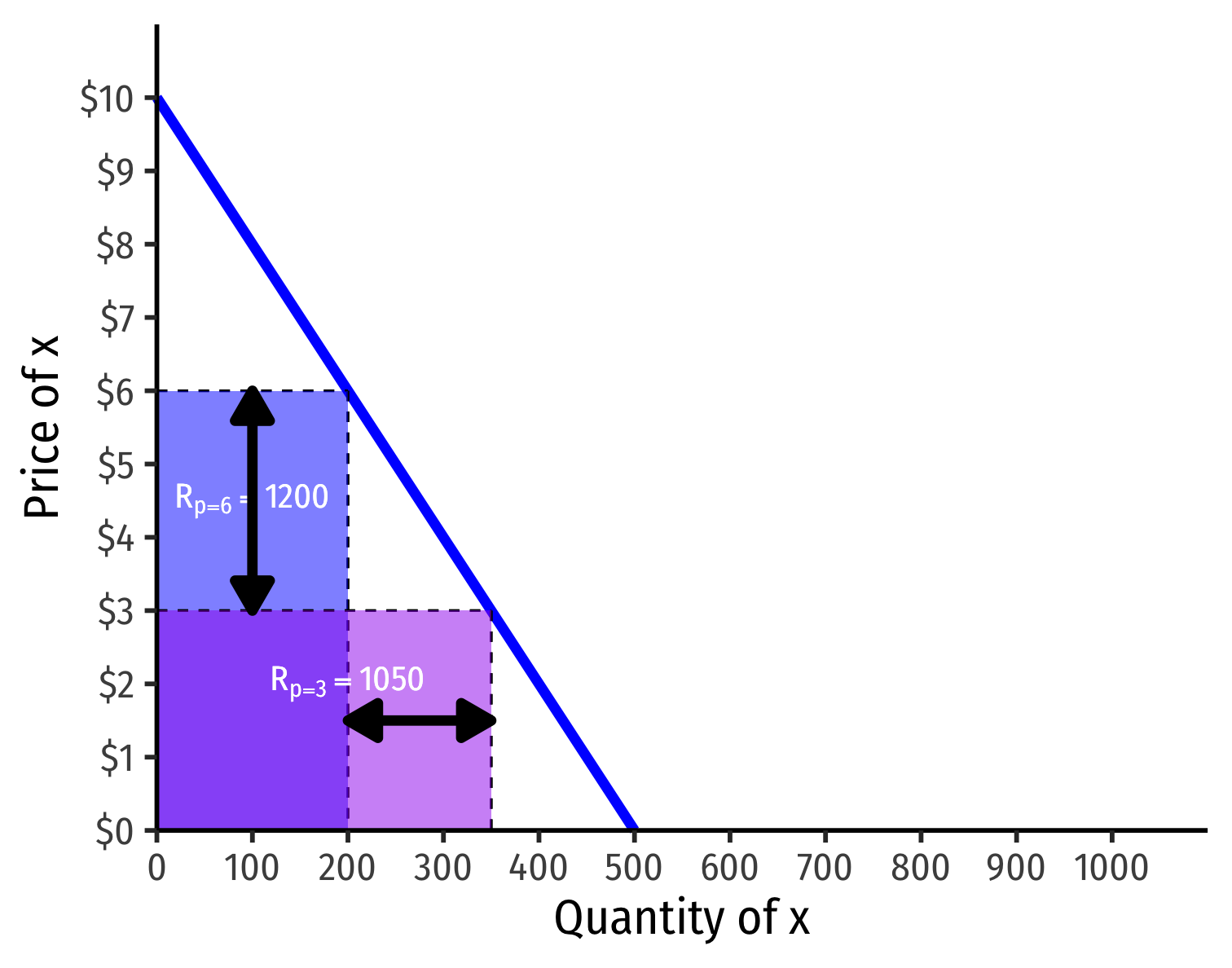
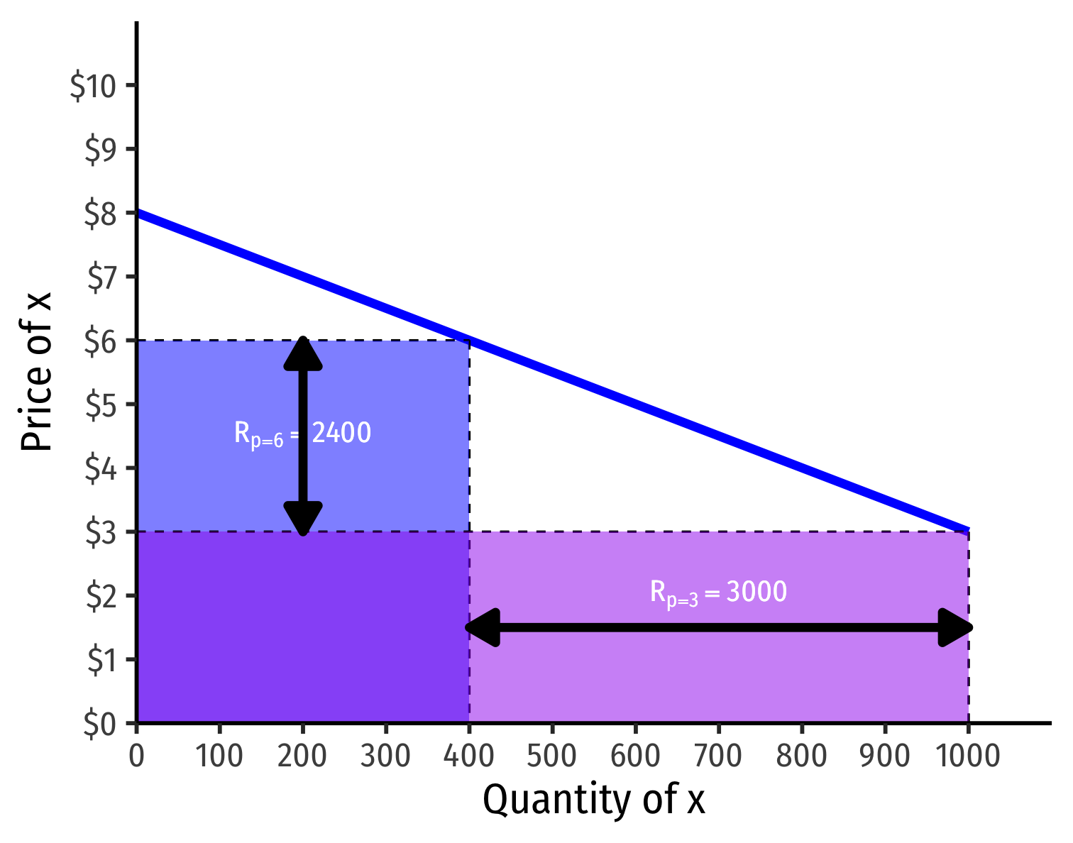
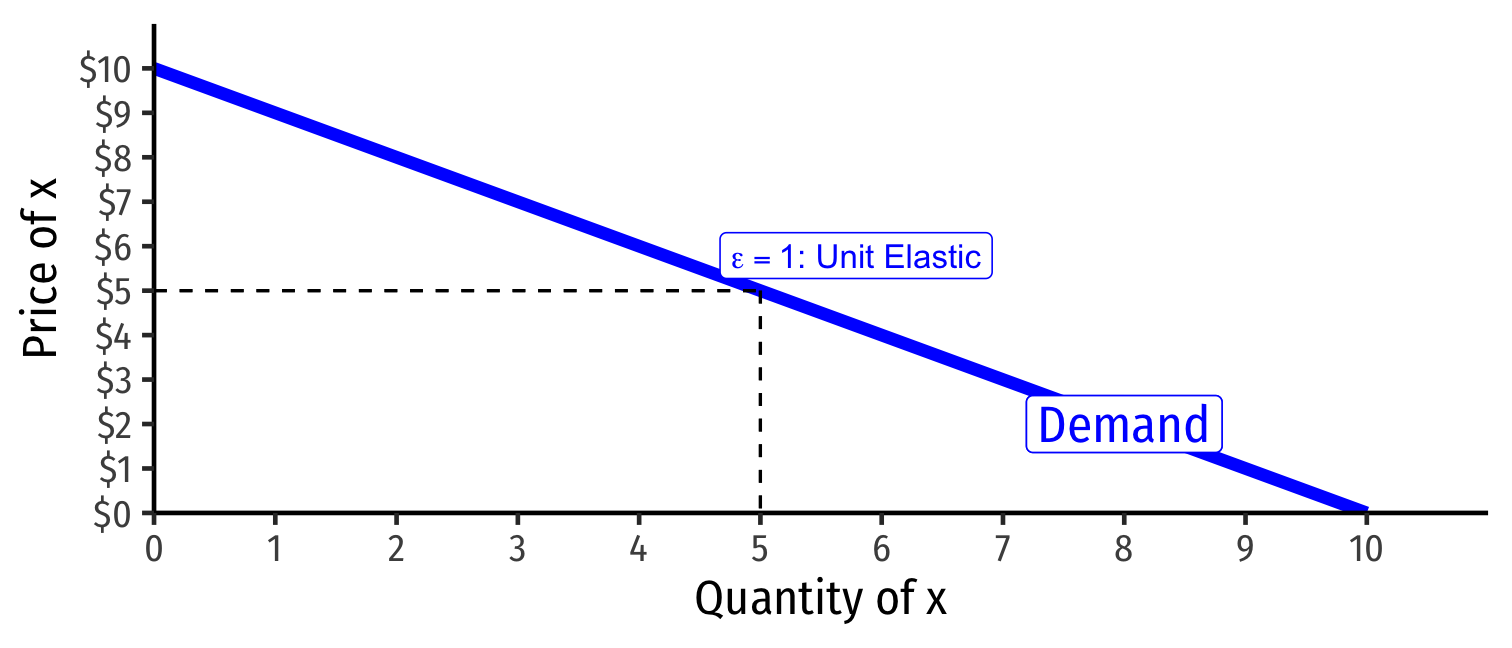
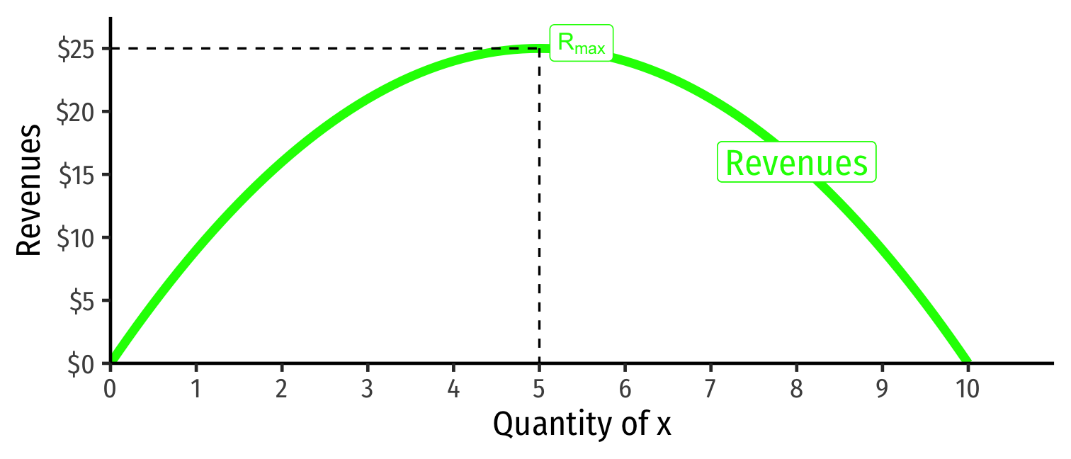
# 1.7 — Price Elasticity

## ECON 306 • Microeconomic Analysis • Spring 2023

### Ryan Safner Associate Professor of Economics <a href="mailto:safner@hood.edu">safner@hood.edu</a> <a href="https://github.com/ryansafner/microS23">ryansafner/microS23</a> <a href="https://microS23.classes.ryansafner.com"> microS23.classes.ryansafner.com</a>

---

# Outline

### [Price Elasticity of Demand](#3)
### [Price Elasticity of Demand and Revenues](#16)
### [Summing Up Unit 1](#32)

---

# Price Elasticity of Demand

---

# Price Elasticity of Demand

- .hi[Price elasticity of demand] measures *how much* (in %) quantity demanded changes in response to a (1%) change in price

`$$\varepsilon_{q_D,p} = \frac{\% \Delta q_D}{\% \Delta p}$$`

]

]

---

# Price Elasticity of Demand: Elastic vs. Inelastic

`$$\varepsilon_{q_D,p} = \frac{\% \Delta q_D}{\% \Delta p}$$`

.smallest[
| | .hi[“Elastic”] | “Unit Elastic” | .hi[“Inelastic”] |
|-----------------|-----------|----------------|------------|
| **Intuitively**: | **Large** response | Proportionate response | **Little** response |
| **Mathematically**: | `$\vert \varepsilon_{q_D,p}\vert > 1$` | `$\vert \varepsilon_{q_D,p}\vert = 1$` | `$\vert \varepsilon_{q_D,p} \vert < 1$` |
| | Numerator `$>$` Denominator | Numerator `$=$` Denominator | Numerator `$<$` Denominator |
| **1% change in `$p$` causes** | **More than 1%** change in `$q_D$` | **Exactly 1%** change in `$q_D$` | **Less than 1%** change in `$q_D$` |

]

---

# Visualizing Price Elasticity of Demand

<img src="1.7-slides_files/figure-html/unnamed-chunk-2-1.png" width="504" style="display: block; margin: auto;" />
]

.center[
.smallest[
“Elastic” Demand Curve
]
]
<img src="1.7-slides_files/figure-html/unnamed-chunk-3-1.png" width="504" style="display: block; margin: auto;" />
]

---

# Price Elasticity of Demand Formula

`$$\varepsilon_{q_D,p} = \frac{\% \Delta q_D}{\% \Delta p}$$`

]

]

---

# Price Elasticity of Demand Formula

`$$\varepsilon_{q,p} = \frac{\% \Delta q}{\% \Delta p} = \cfrac{\left(\frac{\Delta q}{q}\right)}{\left(\frac{\Delta p}{p}\right)}$$`

]

]

---

# Price Elasticity of Demand Formula

`$$\varepsilon_{q,p} = \frac{\% \Delta q}{\% \Delta p} = \cfrac{\left(\frac{\Delta q}{q}\right)}{\left(\frac{\Delta p}{p}\right)} = \frac{\Delta q}{\Delta p} \times \frac{p}{q}$$`

]

]

---

# Price Elasticity of Demand Formula

`$$\varepsilon_{q,p} = \color{#e64173}{\frac{\Delta q}{\Delta p}} \times \color{#44C1C4}{\frac{p}{q}}$$`

- .pink[First term]: *direction* of the effect
  - This is the .hi[price effect]!
  - Always *negative*!

- .turquoise[Second term]: *magnitude* of the effect
  - Will change depending on `$p$` and `$q$`

]

]

---

# Price Elasticity of Demand Formula

`$$\varepsilon_{q,p} = \frac{\Delta q}{\Delta p} \times \frac{p}{q}$$`

- You’ve learned .hi-purple[“arc”]-price elasticity using the .hi-purple[“midpoint formula’] between 2 points

- Here is a more general formula: the .hi-purple[elasticity at any *single* point]!

- We can actually simplify this even more...does the first term remind you of anything?
]

]

---

# Price Elasticity of Demand Formula

`$$\color{red}{\mathbf{\varepsilon_{q,p}} = \mathbf{\frac{1}{slope} \times \frac{p}{q}}}$$`
- First term is actually the inverse of the slope of the inverse demand curve (that we graph)!

- To find the elasticity at any point, we need 3 things:
    1. The price
    2. The associated quantity demanded
    3. The slope of (inverse) demand

]

]

---

# Example

.bg-washed-green.b--dark-green.ba.bw2.br3.shadow-5.ph4.mt5[
.green[**Example**]: The demand for movie tickets in a small town is given by:

`$$q=1000-50p$$`
]

1. Find the inverse demand function.

2. What is the price elasticity of demand at a price of $5.00?

3. What is the price elasticity of demand at a price of $12.00?

4. At what price is demand unit elastic (i.e. `$\varepsilon_{q,p} = -1)$`?

---

# Price Elasticity Changes Along the Demand Curve

<img src="1.7-slides_files/figure-html/unnamed-chunk-4-1.png" width="504" style="display: block; margin: auto;" />
]

`$$\varepsilon_{q,p} = \mathbf{\frac{1}{slope} \times \frac{p}{q}}$$`

- **Elasticity `$\neq$` slope** (but they are related)!

- .hi-purple[Price elasticity changes along the demand curve]

- Gets *less* elastic as  `$\downarrow$` price `$(\uparrow$` quantity )
  - `$\frac{1}{slope}$` is constant
  - `$\frac{p}{q}$` gets smaller as `$\downarrow p$` and `$\uparrow q$`

]

---

# Determinants of Price Elasticity of Demand

.pull-left[
.smallest[
.hi-purple[What determines how responsive your buying behavior is to a price change?]

- More (fewer) .hi[substitutes] `$\implies$` more (less) elastic
  - Larger categories of products (less elastic) vs. specific brand (more elastic)
  - .hi[Necessities] (less elastic) vs. .hi[luxuries] (more elastic)
  - Large (more elastic) vs. small (less elastic) .hi[portion of budget]

- More (less) .hi[time to adjust] `$\implies$` more (less) elastic
]
]

]

---

# Price Elasticity of Demand and Revenues

---

# Price Elasticity of Demand and Revenues

`$$R(q)=pq$$`
]

]

.center[
![](https://www.dropbox.com/s/d95invtrr7ihfu2/revenues.jpg?raw=1)
]
.footnote[.magenta[†] From the buyer’s side, this is .hi[total expenditures].]

]

---

# Price Elasticity of Demand and Revenues

`$$R(q)=pq$$`

| Demand is | `$\Delta R$` and `$\Delta p$` |
|-----------------------:|---------------------------|
| Elastic `$\vert \varepsilon \vert > 1$` | p & R change **opposite** |
| Unit Elastic `$\vert \varepsilon \vert = 1$` | R **maximized** |
| Inelastic `$\vert \varepsilon \vert < 1$` | p & R change **together** |

]
]

.center[
![](https://www.dropbox.com/s/d95invtrr7ihfu2/revenues.jpg?raw=1)
]
.footnote[.magenta[†] From the buyer’s side, this is .hi[total expenditures].]

]

---

# Price Elasticity of Demand and Revenues

`$$R(q)=pq$$`

]
]

---

# Revenues: Example I

---

# Revenues: Example I

---

# Revenues: Example II

---

# Revenues: Example II

---

# Visualizing Price Elasticity of Demand and Revenues

(Agricultural Products)
]
]
<img src="1.7-slides_files/figure-html/unnamed-chunk-9-1.png" width="504" style="display: block; margin: auto;" />
]

(Computer Chips)
]
]
<img src="1.7-slides_files/figure-html/unnamed-chunk-10-1.png" width="504" style="display: block; margin: auto;" />
]

---

# Price Elasticity and Revenues

`$$R(q)=pq$$`

| `$q$` | `$p$` | `$R(q)$` |
|----:|----:|----:|
| 0 | 10 | 0 | 
| 1 | 9 | 9 | 
| 2 | 8 | 16 | 
| 3 | 7 | 21 | 
| 4 | 6 | 24 | 
| **5** | **5** | **25** | 
| 6 | 4 | 24 | 
| 7 | 3 | 21 | 
| 8 | 2 | 16 |
| 9 | 1 | 9 |
| 10 | 0 | 0 |

]
]

---

# Price Elasticity and Revenues: Example I

.pull-left[
.center[
![:scale 80%](https://www.dropbox.com/s/ocf4pojybur3fy6/buildabearelasticity.png?raw=1)

Source: [CNN (July 2, 2018)](https://www.cnn.com/2018/07/12/us/build-a-bear-lines/)

]

> "Build-A-Bear announced its Pay Your Age event earlier this week. Customers who show up to the stores can pay their current age for the popular stuffed animals. On Wednesday, the retailer wrote on its Facebook page that it was 'anticipating potential of long lines and wait times.'"

]

---

# Price Elasticity and Revenues: Example II

.pull-left[
.center[
![:scale 80%](https://www.dropbox.com/s/wt77kiwckzgcvbx/superbowlelasticity.png?raw=1)

Source: [Wall Street Journal (Feb 3, 2019)](https://www.wsj.com/articles/as-nfl-courts-fans-in-stands-atlanta-is-king-11549201747)
]

]

.pull-right[
.smallest[
"While leaguewide average attendance dropped .43% this season to its lowest level since 2010, Atlanta’s attendance rose for the second season. Mercedes-Benz Stadium and the Falcons have become the model for drawing fans and keeping them happy."

"Instead of charging elevated sums—a long-held industry practice that fans despised—the Falcons would price most of its food at what it sold for on the street...**Prices plunged 50%.** Fans rejoiced. **Although the team made less money on each $2 hot dog it sold, it made more overall.** Average fan spending per game rose 16%. Atlanta’s food services, which ranked 18th in the NFL in the 2016 annual league survey, shot up to No. 1 in 2017 in every metric—and by a wide margin."
]
]

---

# Price Elasticity and Revenues: Example III

Cowen & Tabarrok (2014: p.75)
]

---

# Price Elasticity and Revenues: Example IV

---

# Summing Up Unit 1

---

# Models of Individual Choice I

> "All models are lies. The art is telling useful lies." - George Box

- Remember, we're not modelling the **process** by which people **actually** choose

- We're **predicting consequences** (in people's choices) when **parameters change**

]

---

# Models of Individual Choice II

- Constrained optimization models are the **main** workhorse model in economics

- All constrained optimization models have three moving parts:

1. **Choose:** .blue[ < some alternative >]

2. **In order to maximize:** .green[< some objective >]

3. **Subject to:** .red[< some constraints >]

]

.pull-right[
.center[
![:scale 100%](https://www.dropbox.com/s/qvr240t5j6t3arm/optimize.jpeg?raw=1)
]
]

---

# Models of Individual Choice III

---

# Applications of Consumer Theory

- See today's [class notes page](/content/1.7-content) for some applications of consumer theory:

1. **Uncertainty**: risky outcomes & insurance

2. **Exchange**: two individuals trading their endowments, general equilibrium, & Pareto efficiency

3. **Taxes**: Which is better for consumers, a consumption tax or a (revenue-equivalent) income tax?

4. **Intertemporal choice**: saving, borrowing, lending, & interest