2.3 — Cost Minimization
ECON 306 • Microeconomic Analysis • Spring 2023
Ryan Safner
Associate Professor of Economics
safner@hood.edu
ryansafner/microS23
microS23.classes.ryansafner.com
Recall: The Firm's Two Problems
1st Stage: firm's profit maximization problem:
Choose: < output >
In order to maximize: < profits >
- We'll cover this later...first we'll explore:
2nd Stage: firm's cost minimization problem:
Choose: < inputs >
In order to minimize: < cost >
Subject to: < producing the optimal output >
- Minimizing costs ⟺ maximizing profits

Solving the Cost Minimization Problem
The Firm's Cost Minimization Problem
- The firm's cost minimization problem is:
Choose: < inputs: l,k>
In order to minimize: < total cost: wl+rk >
Subject to: < producing the optimal output: q∗=f(l,k) >

The Cost Minimization Problem: Tools
Our tools for firm's input choices:
Choice: combination of inputs (l,k)
Production function/isoquants: firm's technological constraints
- How the firm trades off between inputs
- Isocost line: firm's total cost (for given output and input prices)
- How the market trades off between inputs

The Cost Minimization Problem: Verbally
- The firms's cost minimization problem:
choose a combination of l and k to minimize total cost that produces the optimal amount of output

The Cost Minimization Problem: Math
minl,kwl+rk s.t.q∗=f(l,k)
- This requires calculus to solve. We will look at graphs instead!

The Firm's Least-Cost Input Combination: Graphically
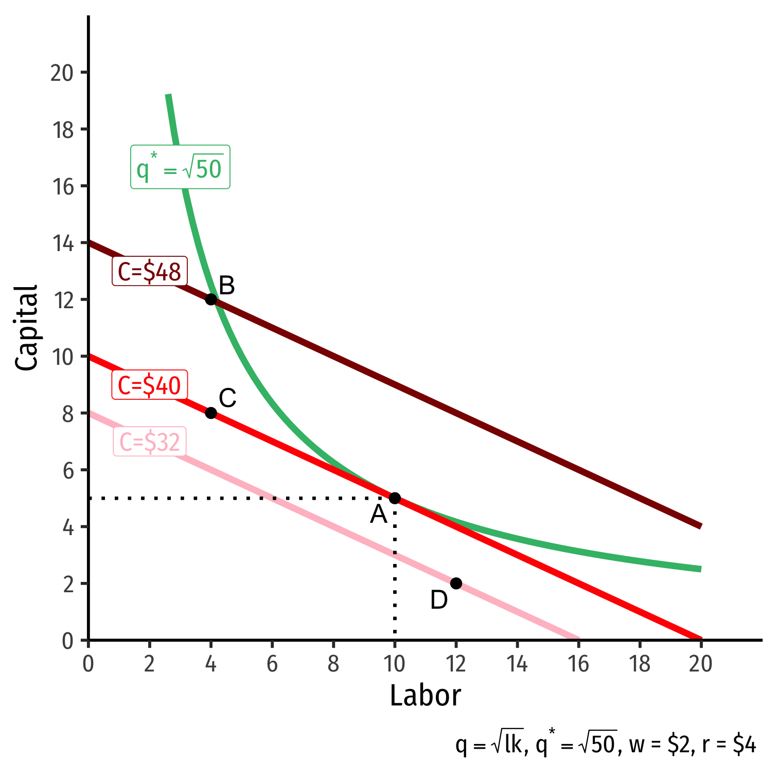
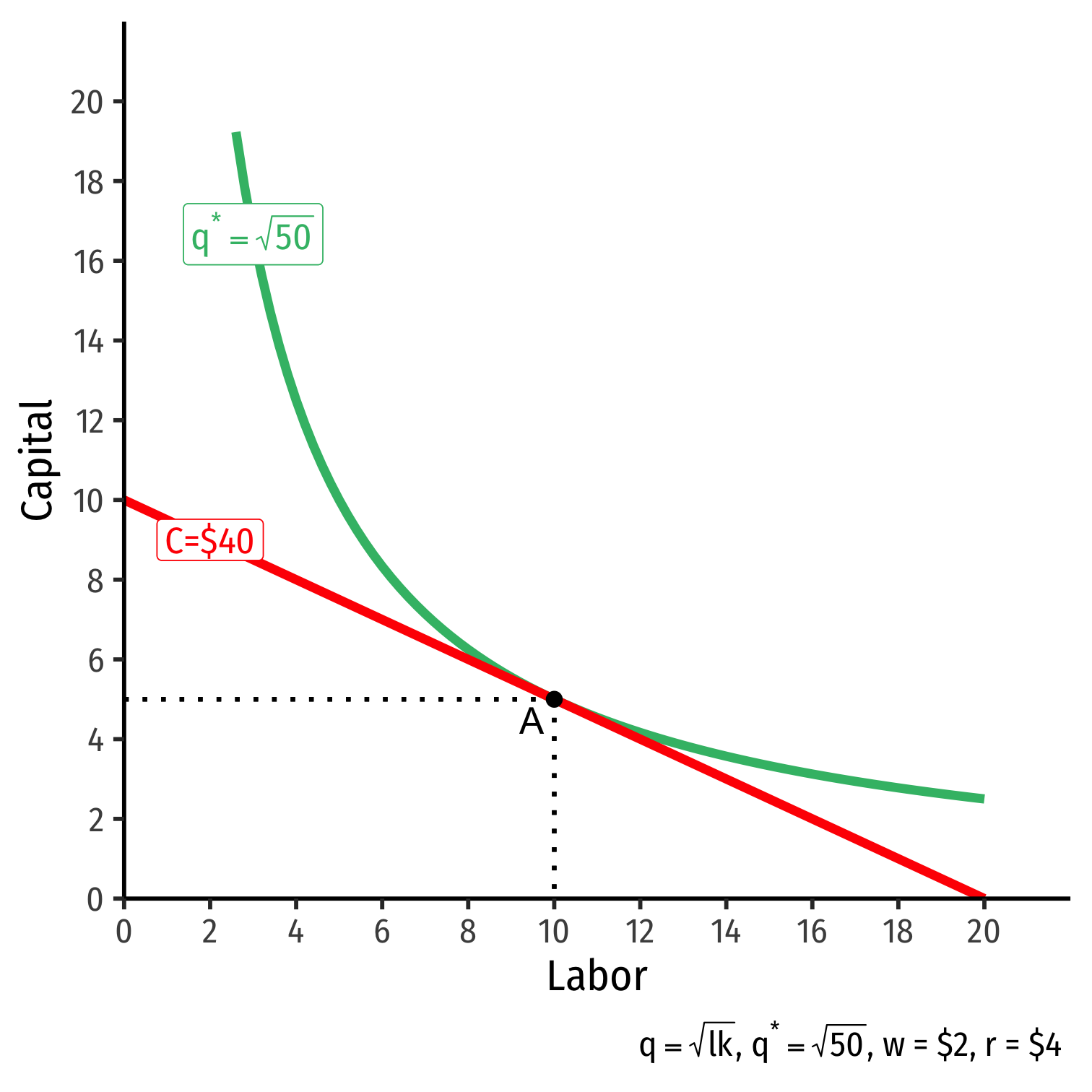
- Graphical solution: Lowest isocost line tangent to desired isoquant (A)

The Firm's Least-Cost Input Combination: Graphically
Graphical solution: Lowest isocost line tangent to desired isoquant (A)
B produces same output as A, but higher cost
C is same cost as A, but does not produce desired output
D is cheaper, does not produce desired output

The Firm's Least-Cost Input Combination: Why A?
Isoquant curve slope=Isocost line slope

The Firm's Least-Cost Input Combination: Why A?
Isoquant curve slope=Isocost line slopeMRTSl,k=wrMPlMPk=wr0.5=0.5
Marginal benefit = Marginal cost
- Firm would exchange at same rate as market
No other combination of (l,k) exists at current prices & output that could produce q⋆ at lower cost!

Two Equivalent Rules
Rule 1
MPlMPk=wr
- Easier for calculation (slopes)

Two Equivalent Rules
Rule 1
MPlMPk=wr
- Easier for calculation (slopes)
Rule 2
MPlw=MPkr
- Easier for intuition (next slide)

The Equimarginal Rule Again I
MPlw=MPkr=⋯=MPnpn
Equimarginal Rule: the cost of production is minimized where the marginal product per dollar spent is equalized across all n possible inputs
Firm will always choose an option that gives higher marginal product (e.g. if MPl>MPk)
- But each option has a different cost, so we weight each option by its price, hence MPnpn
The Equimarginal Rule Again II
Any optimum in economics: no better alternatives exist under current constraints
No possible change in your inputs to produce q∗ that would lower cost

The Firm's Least-Cost Input Combination: Example
Example:
Your firm can use labor l and capital k to produce output according to the production function: q=2lk
The marginal products are:
MPl=2kMPk=2l
You want to produce 100 units, the price of labor is $10, and the price of capital is $5.
- What is the least-cost combination of labor and capital that produces 100 units of output?
- How much does this combination cost?
Returns to Scale
Returns to Scale
- The returns to scale of production: change in output when all inputs are increased at the same rate (scale)

Returns to Scale
The returns to scale of production: change in output when all inputs are increased at the same rate (scale)
Constant returns to scale: output increases at same proportionate rate to inputs change
- e.g. double all inputs, output doubles

Returns to Scale
The returns to scale of production: change in output when all inputs are increased at the same rate (scale)
Constant returns to scale: output increases at same proportionate rate to inputs change
- e.g. double all inputs, output doubles
Increasing returns to scale: output increases more than proportionately to inputs change
- e.g. double all inputs, output more than doubles

Returns to Scale
The returns to scale of production: change in output when all inputs are increased at the same rate (scale)
Constant returns to scale: output increases at same proportionate rate to inputs change
- e.g. double all inputs, output doubles
Increasing returns to scale: output increases more than proportionately to inputs change†
- e.g. double all inputs, output more than doubles
Decreasing returns to scale: output increases less than proportionately to inputs change
- e.g. double all inputs, output less than doubles

† See my new newsletter Increasing Returns for more on the importance of this idea
Returns to Scale: Example
Example: Do the following production functions exhibit constant returns to scale, increasing returns to scale, or decreasing returns to scale?
q=4l+2k
q=2lk
q=2l0.3k0.3
Returns to Scale: Cobb-Douglas
One reason Cobb-Douglas functions are great: easy to determine returns to scale:
q=Akαlβα+β=1: constant returns to scale
- α+β>1: increasing returns to scale
α+β<1: decreasing returns to scale
Note this trick only works for Cobb-Douglas functions!

Cobb-Douglas: Constant Returns Case
A common case of Cobb-Douglas is often written as:
q=Akαl1−α (i.e., the exponents sum to 1, constant returns)α is the output elasticity of capital
- A 1% increase in k leads to an α% increase in q
1−α is the output elasticity of labor
- A 1% increase in l leads to a (1−α)% increase in q

Output-Expansion Paths & Cost Curves

Goolsbee et. al (2011: 246)
Output Expansion Path: curve illustrating the changes in the optimal mix of inputs and the total cost to produce an increasing amount of output
Total Cost curve: curve showing the total cost of producing different amounts of output (next class)
See next class' notes page to see how we go from our least-cost combinations over a range of outputs to derive a total cost function