2.5 — Short Run Profit Maximization

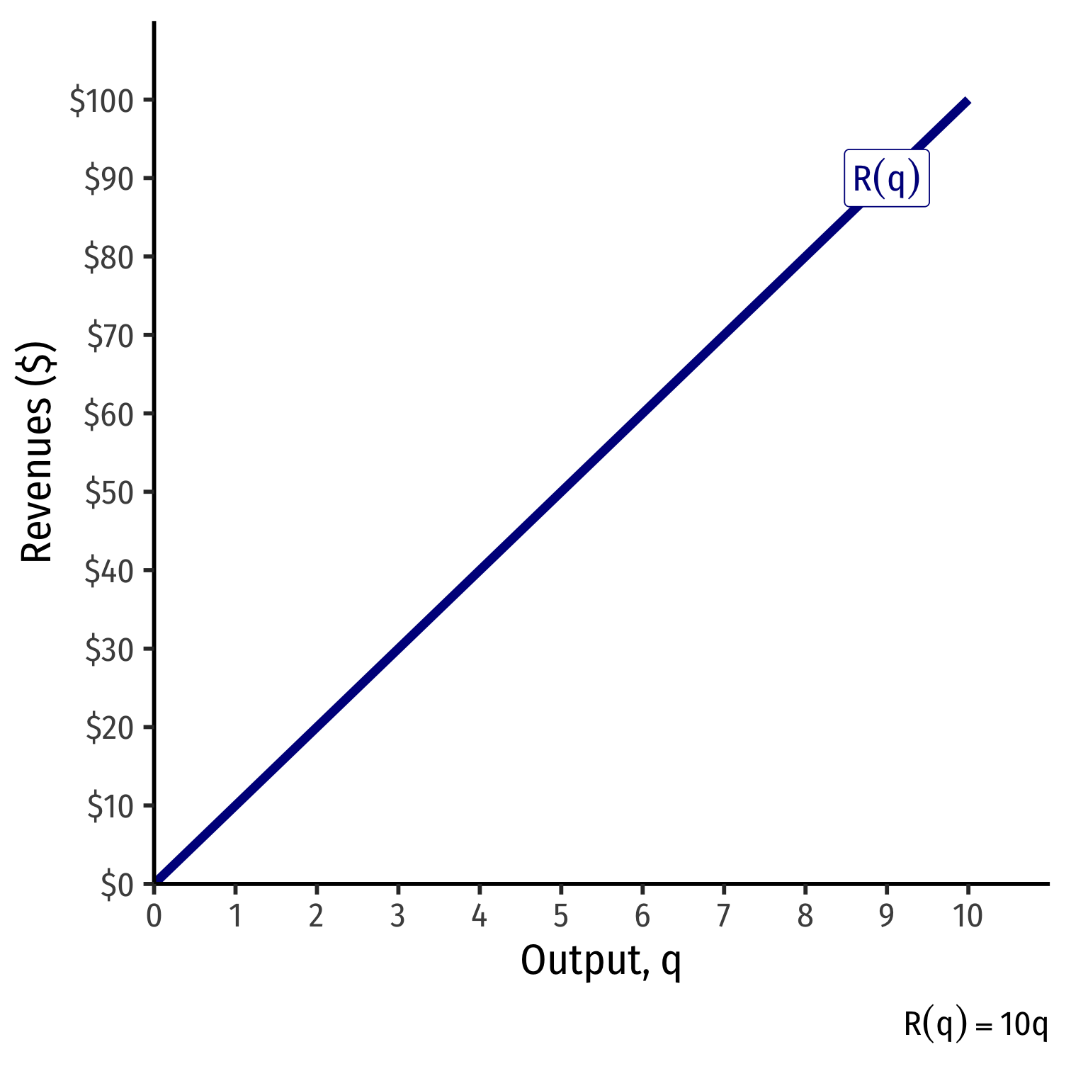
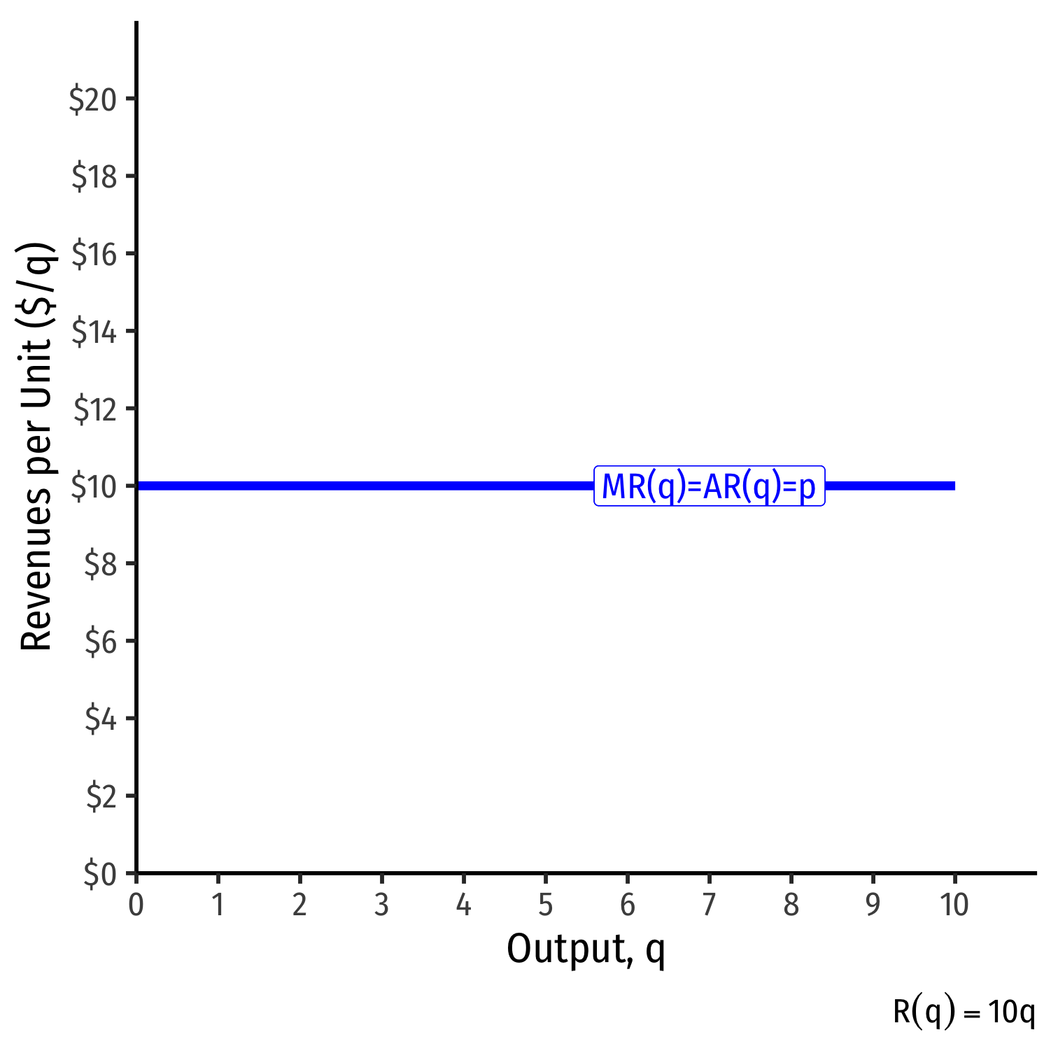
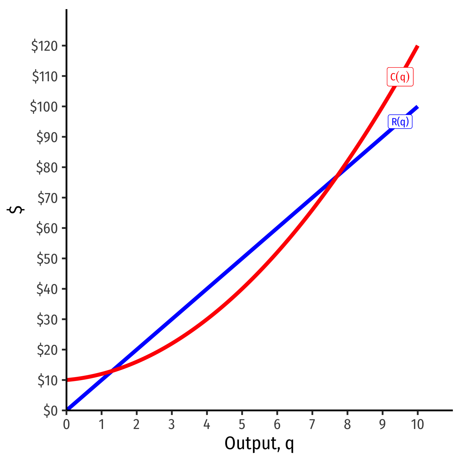
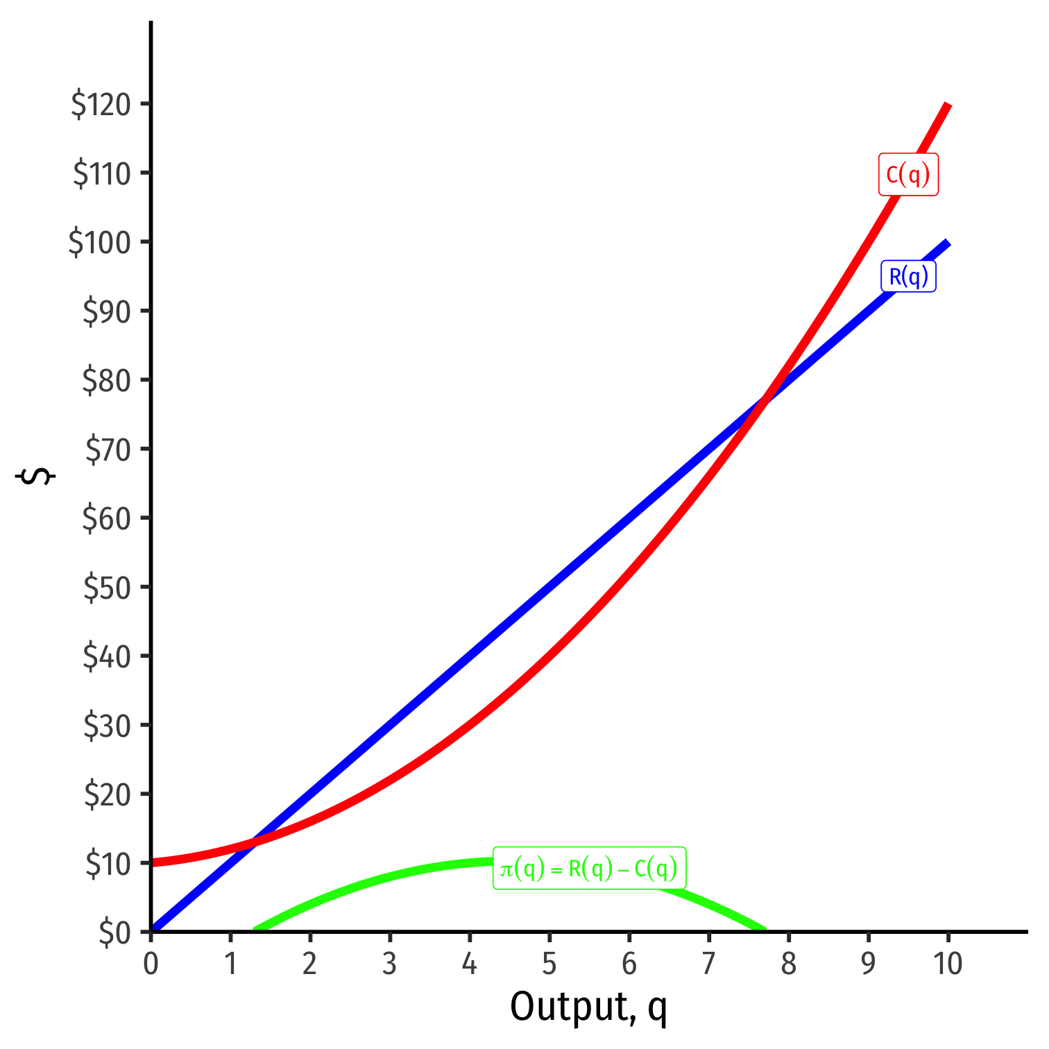
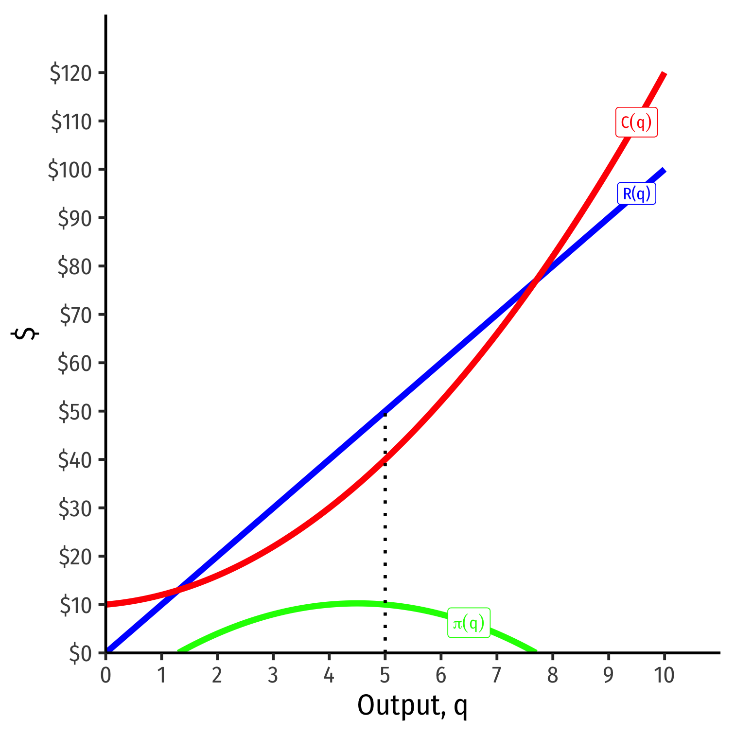
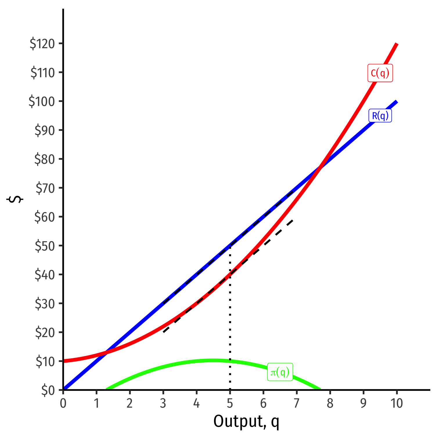
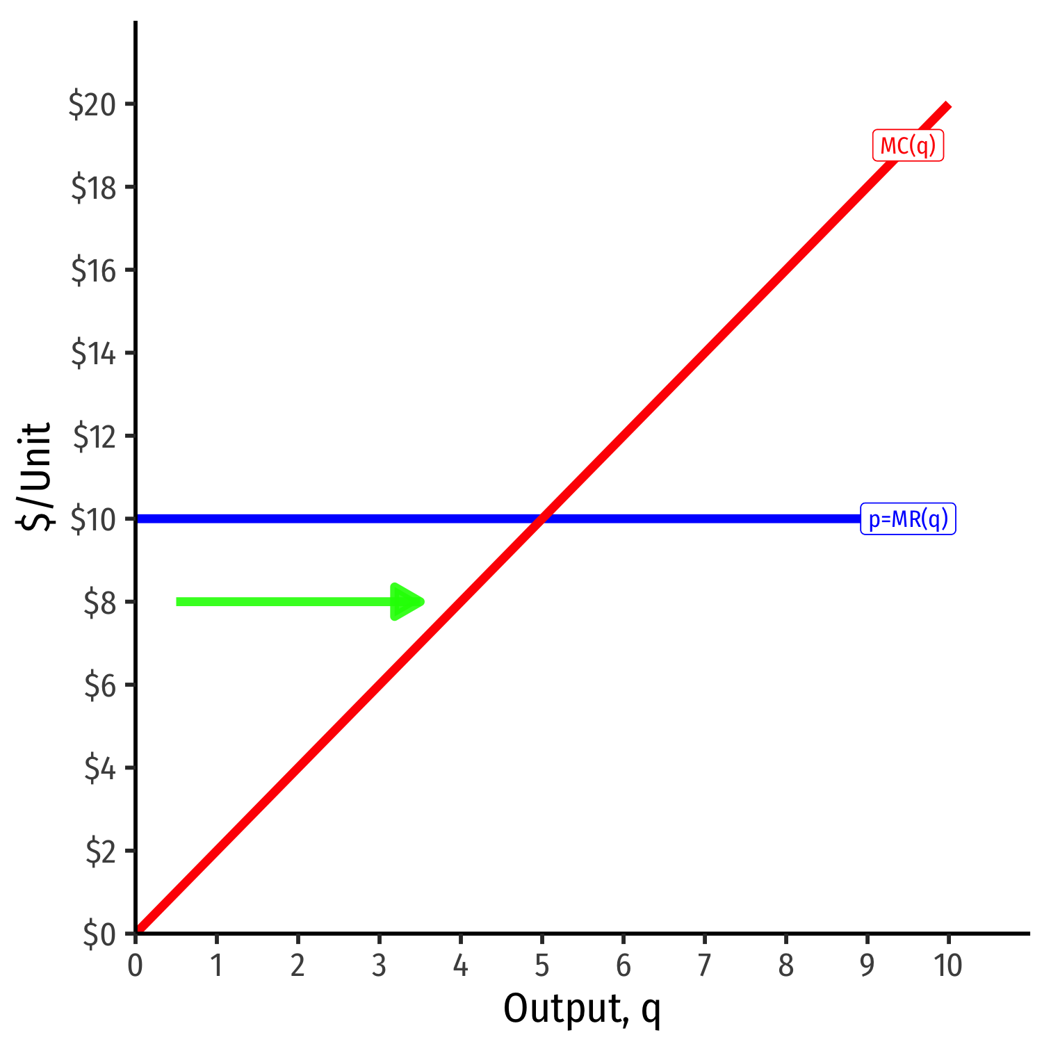
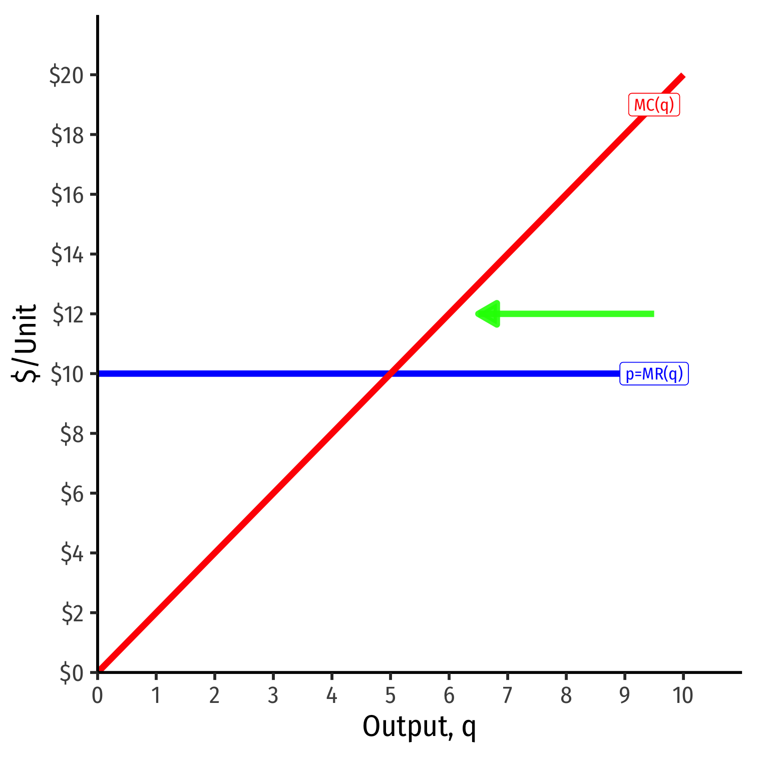
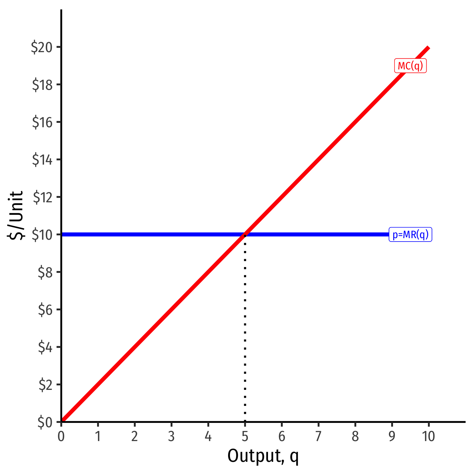
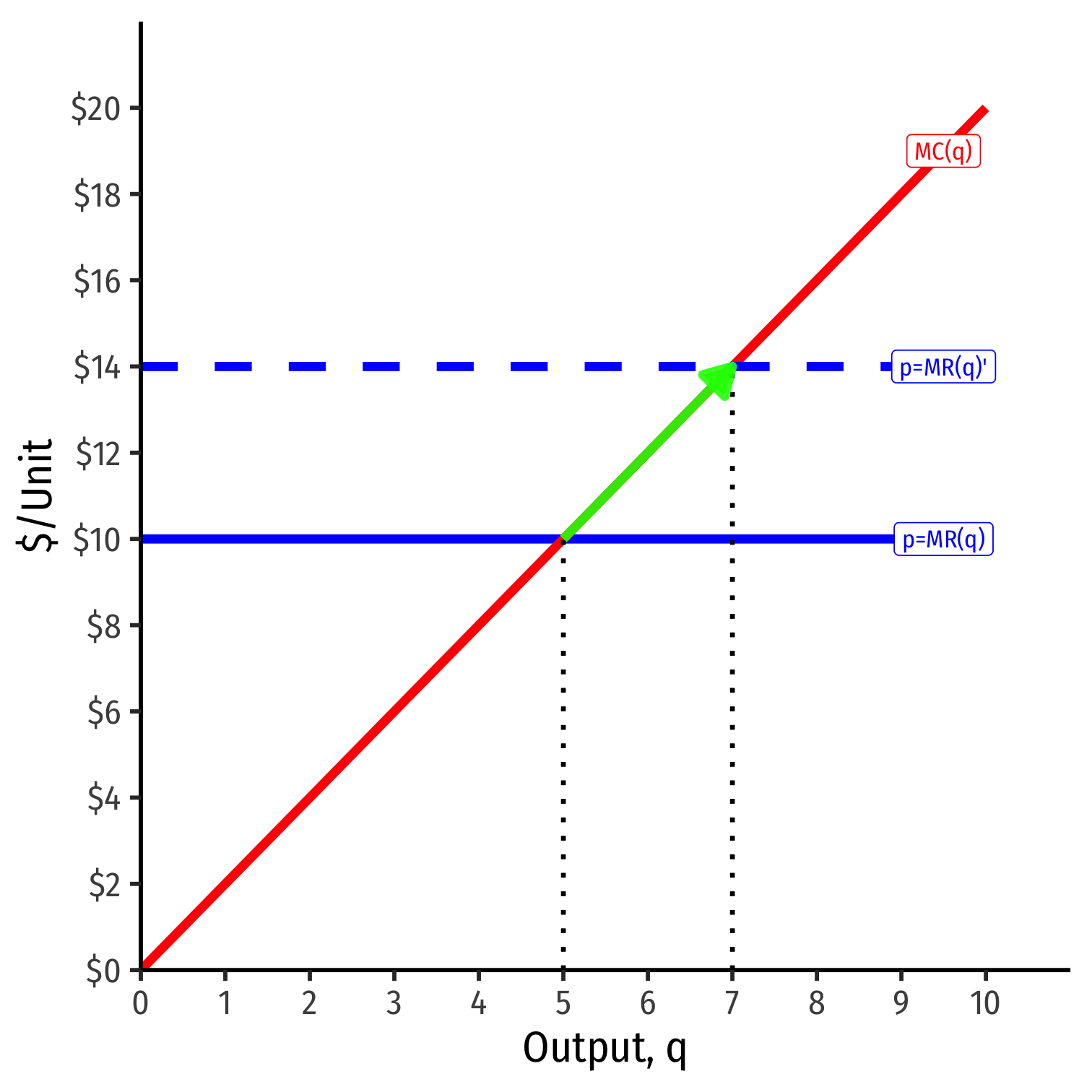
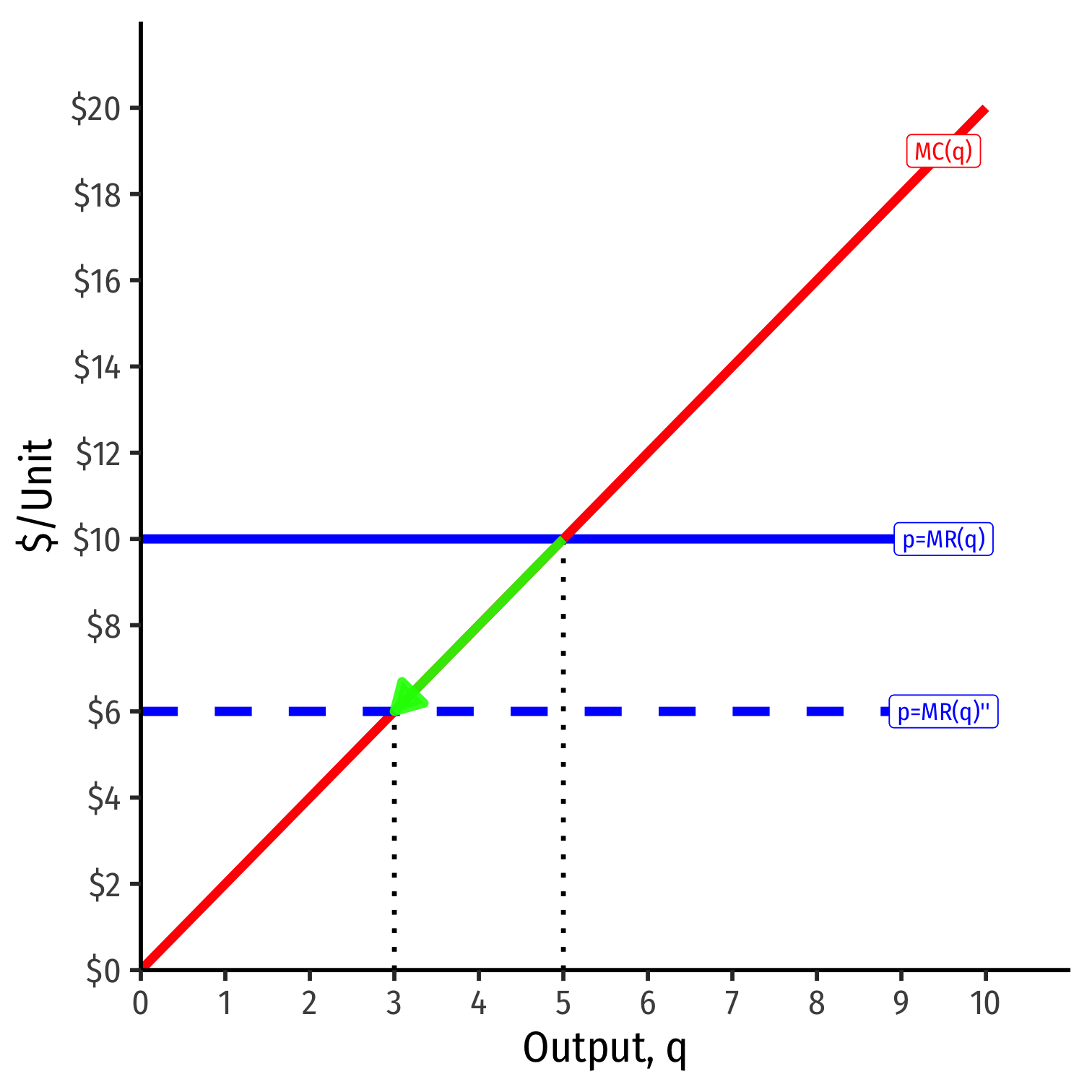
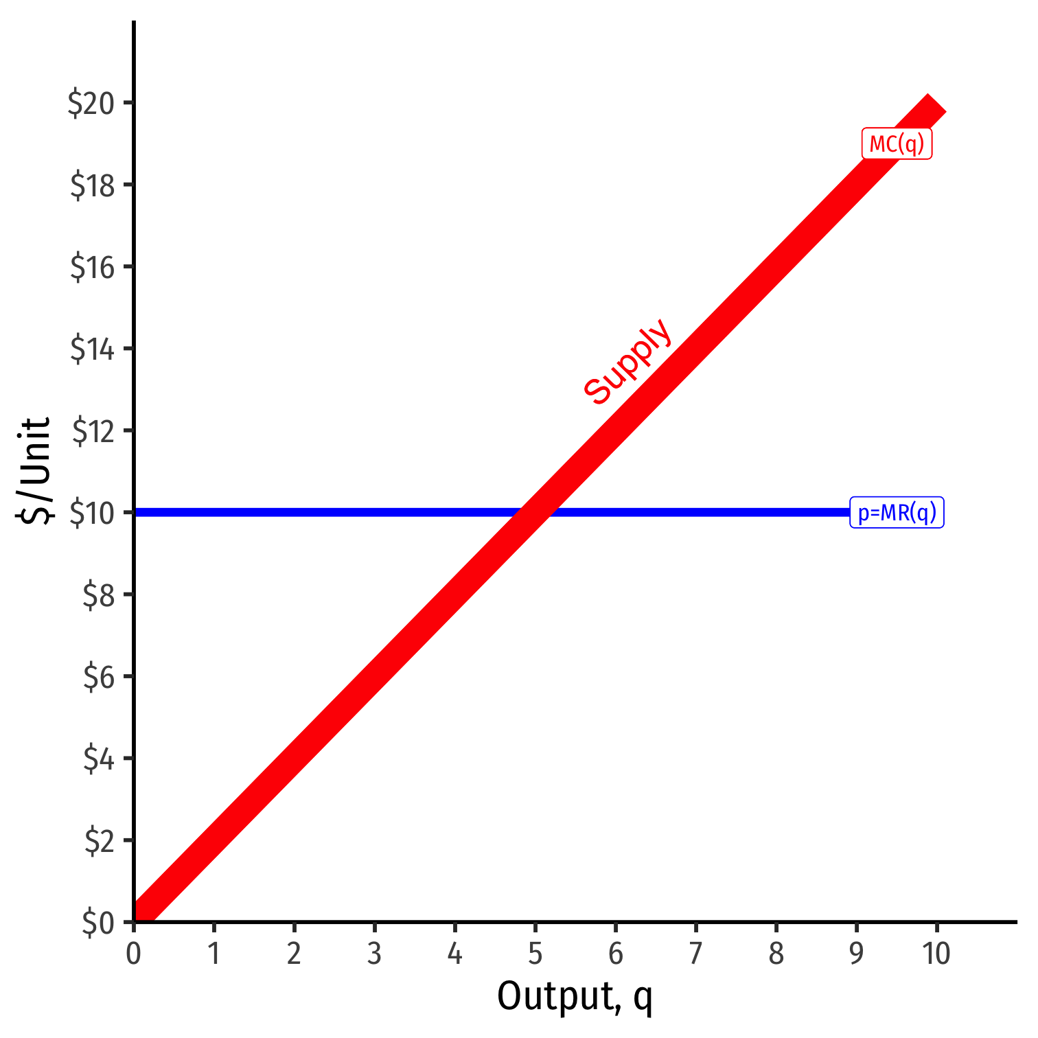
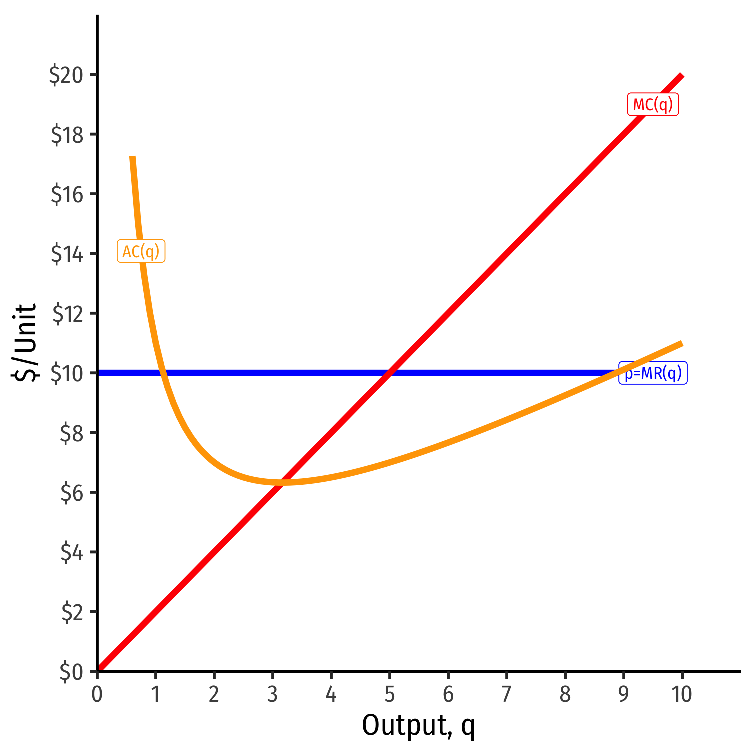
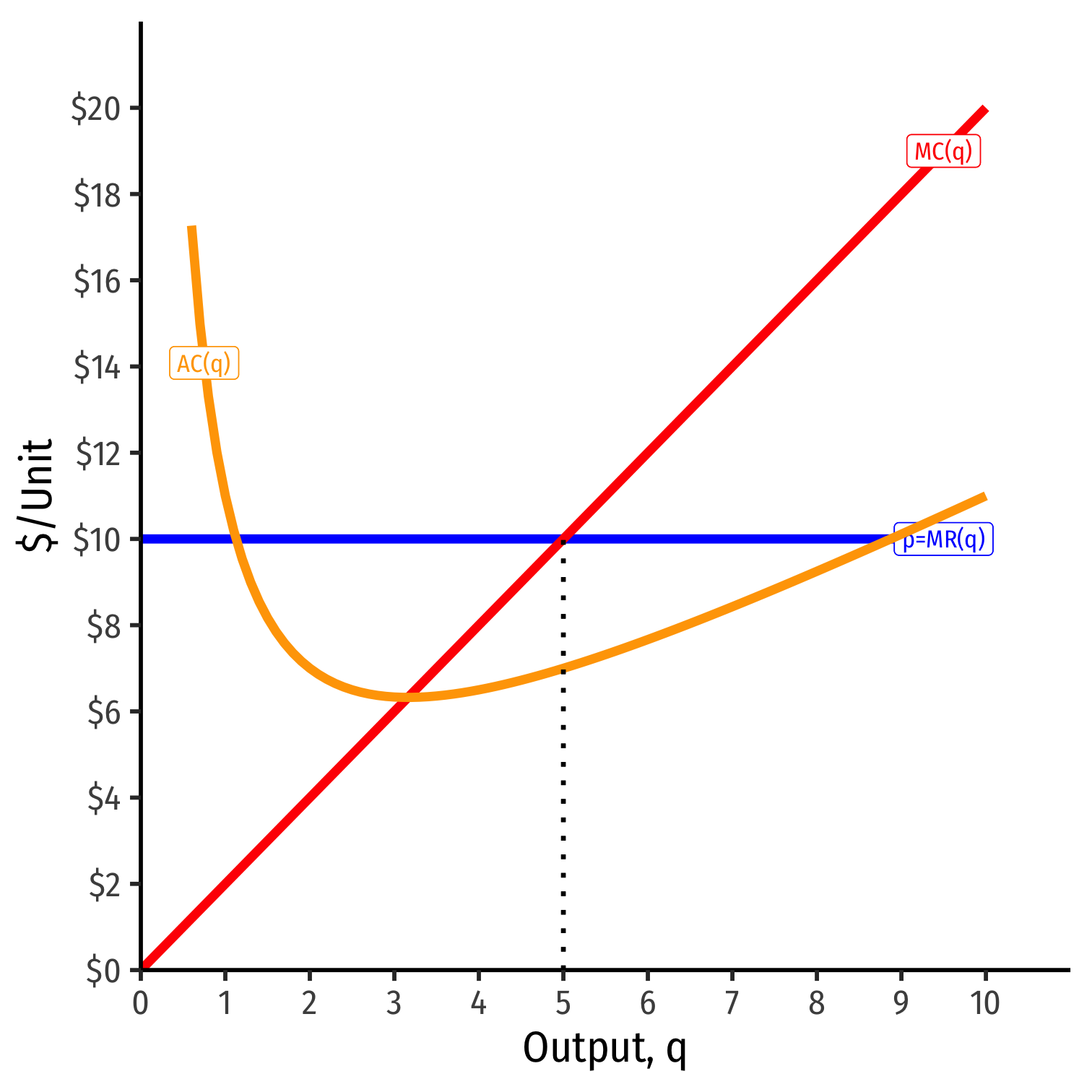
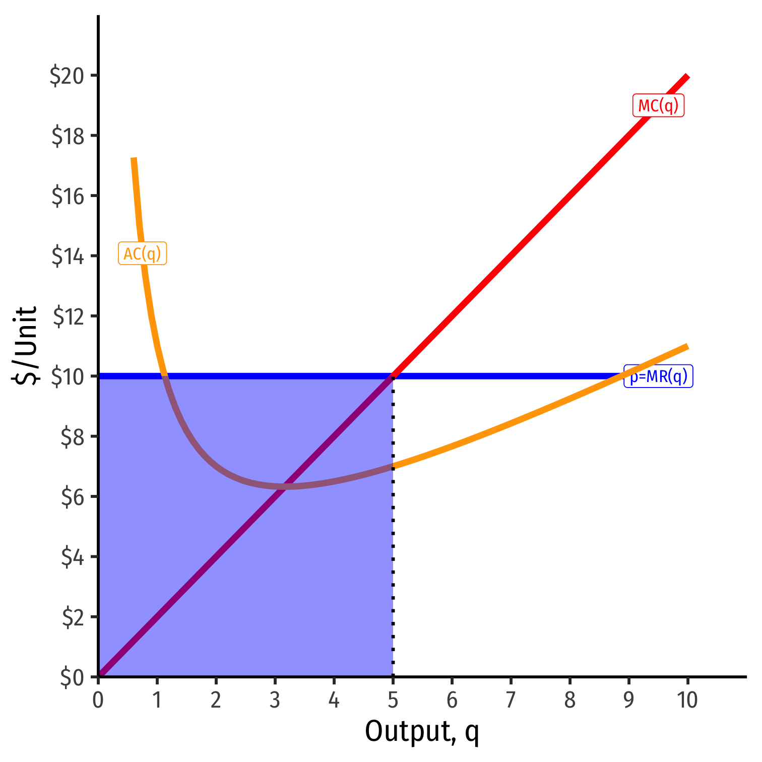
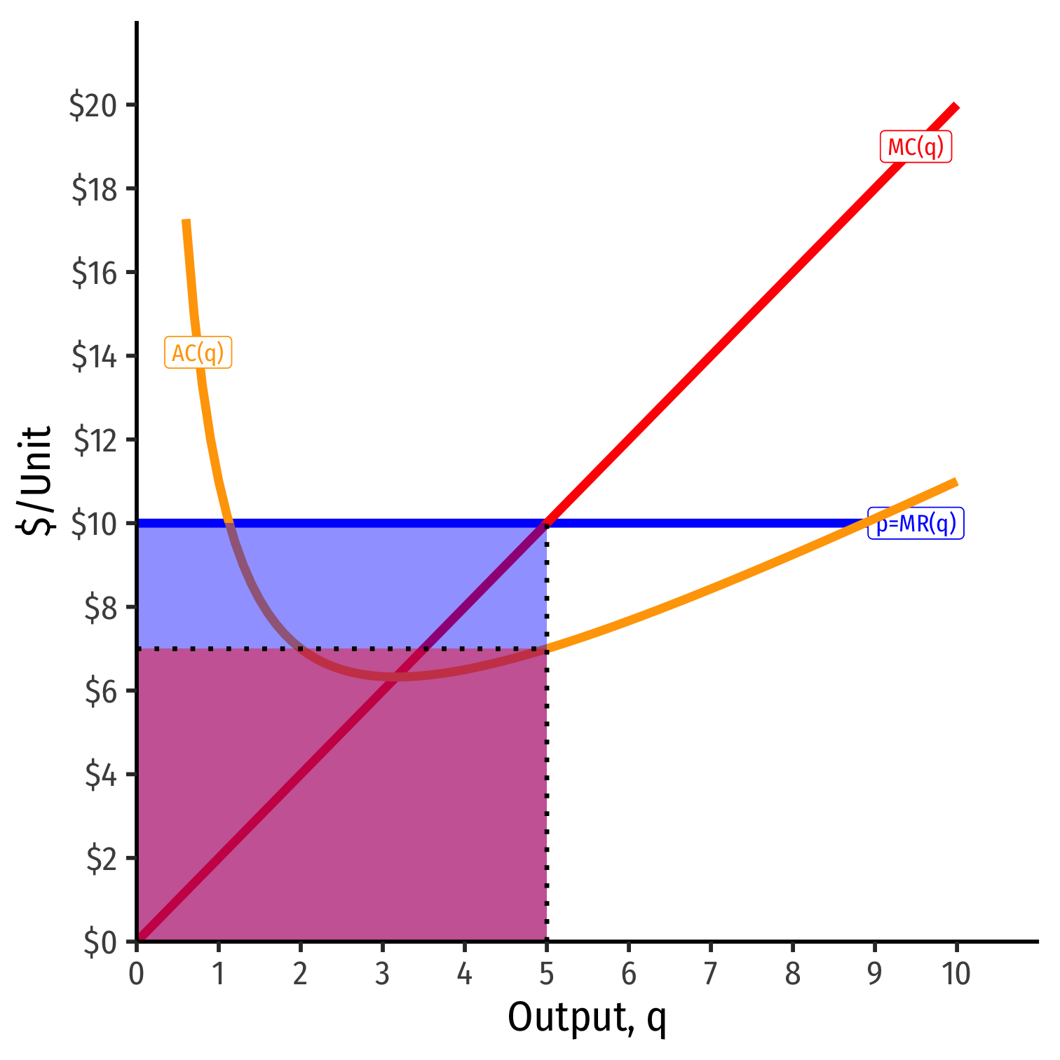
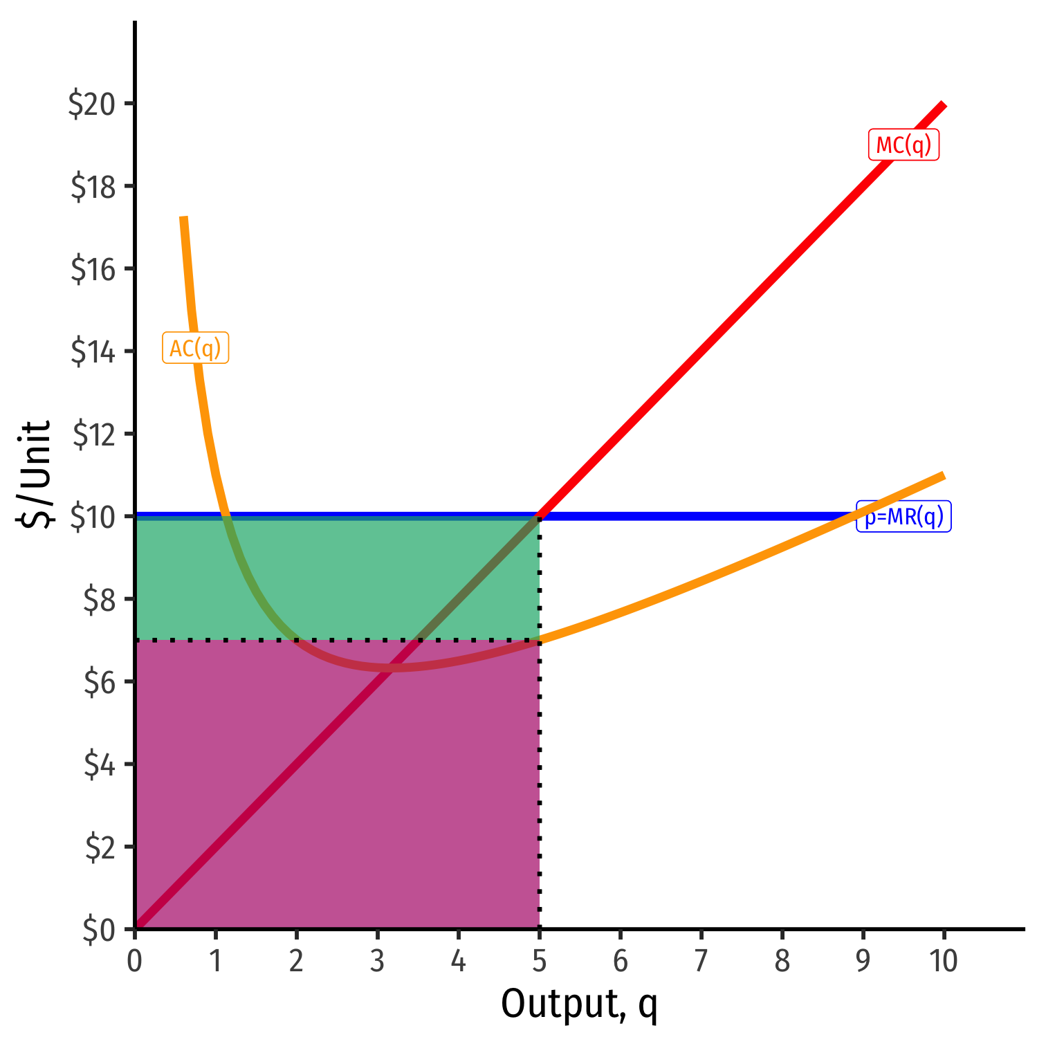
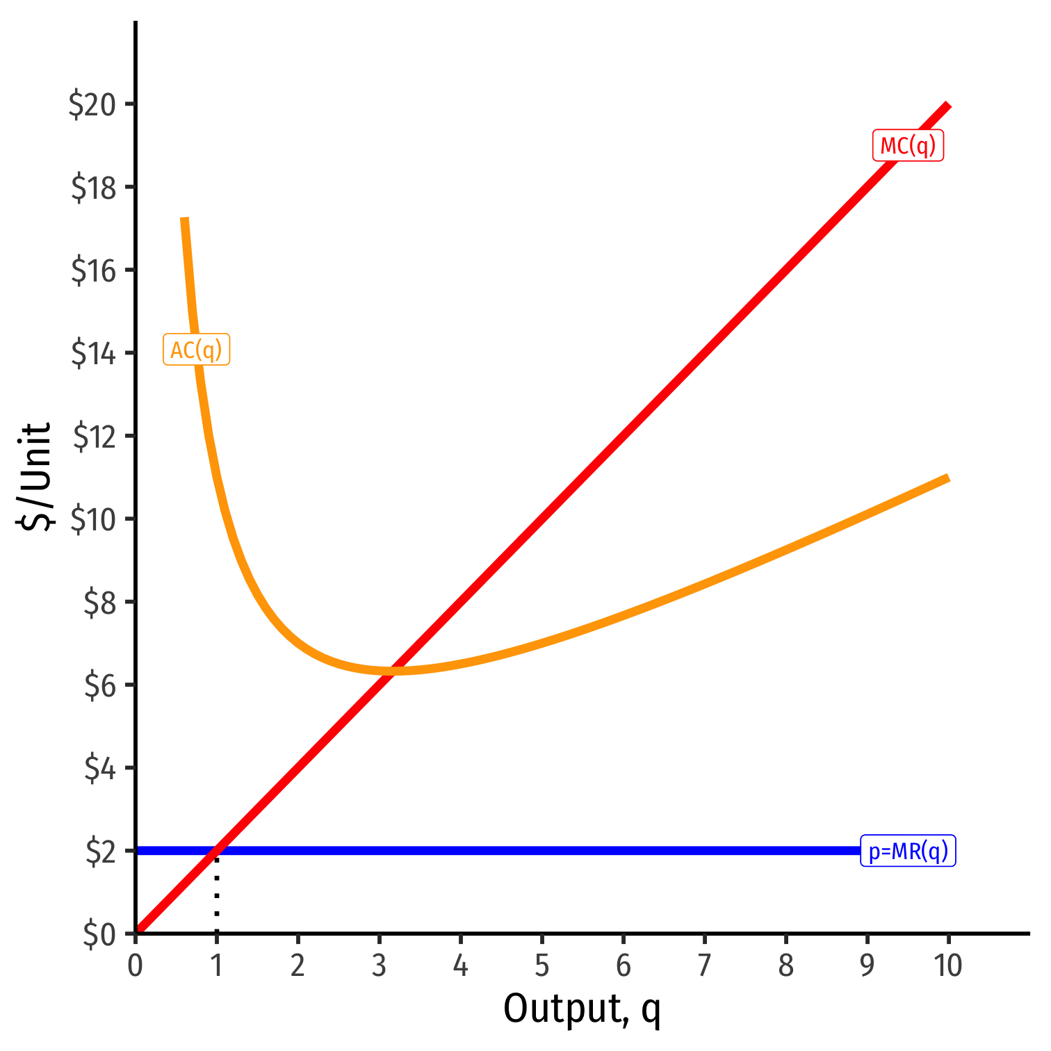
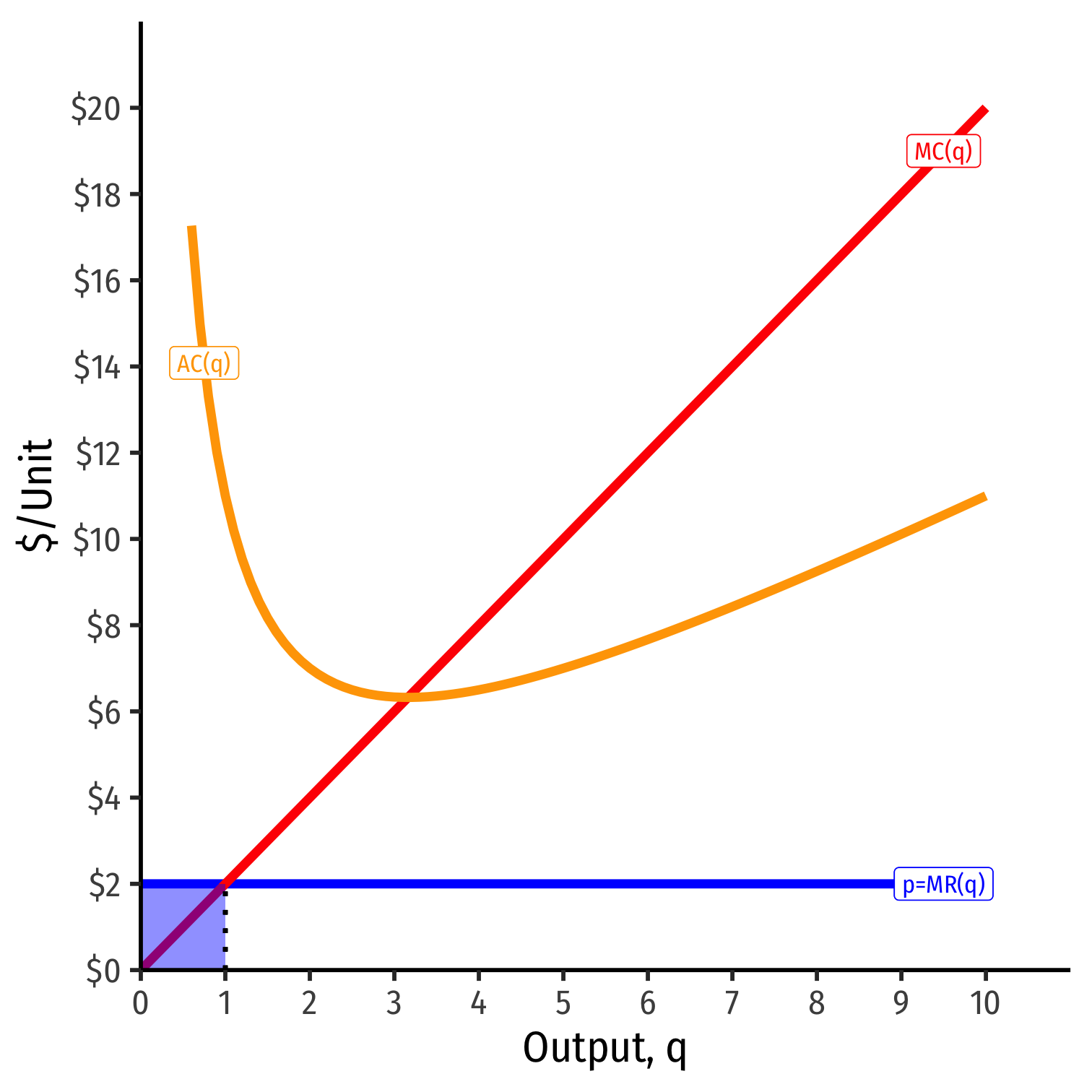
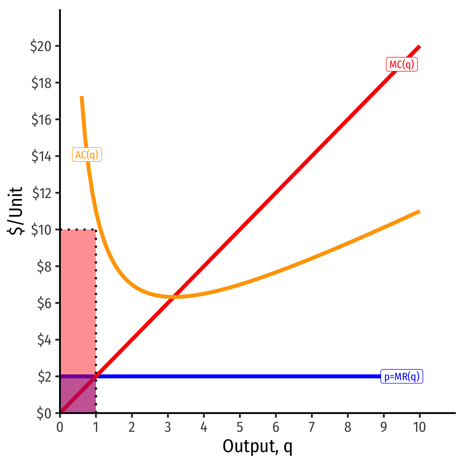
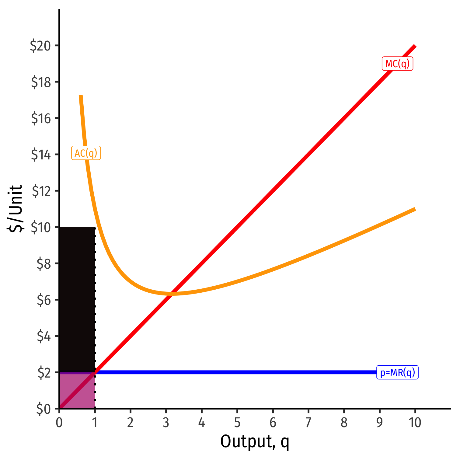
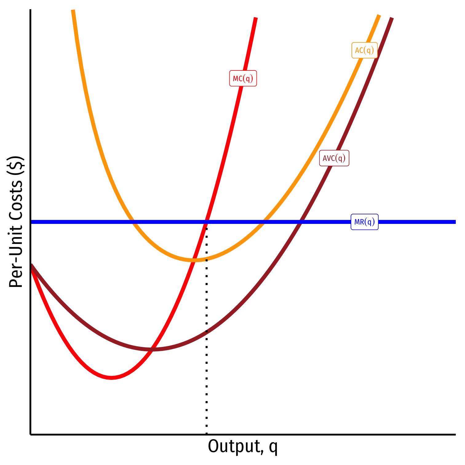
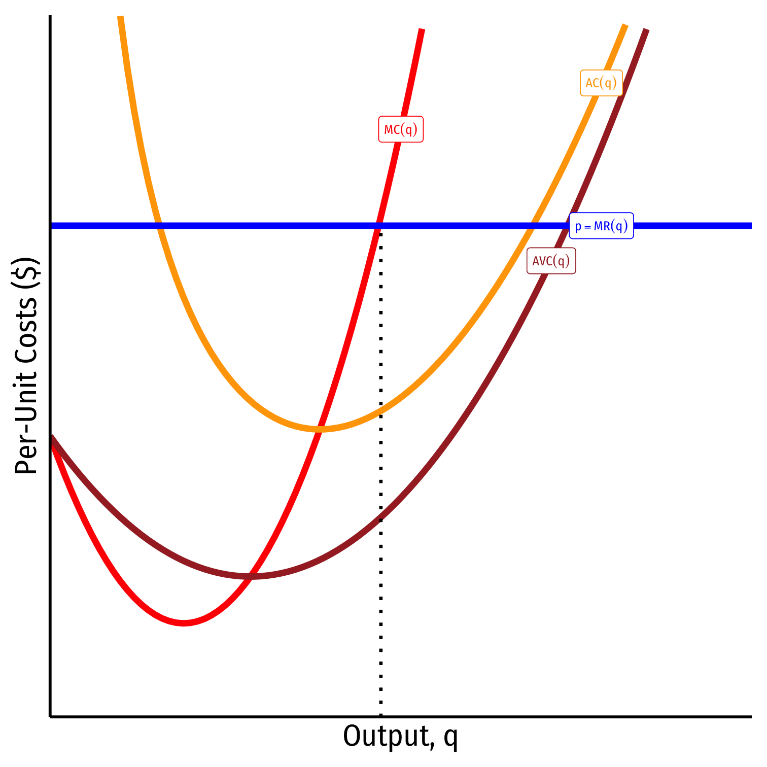
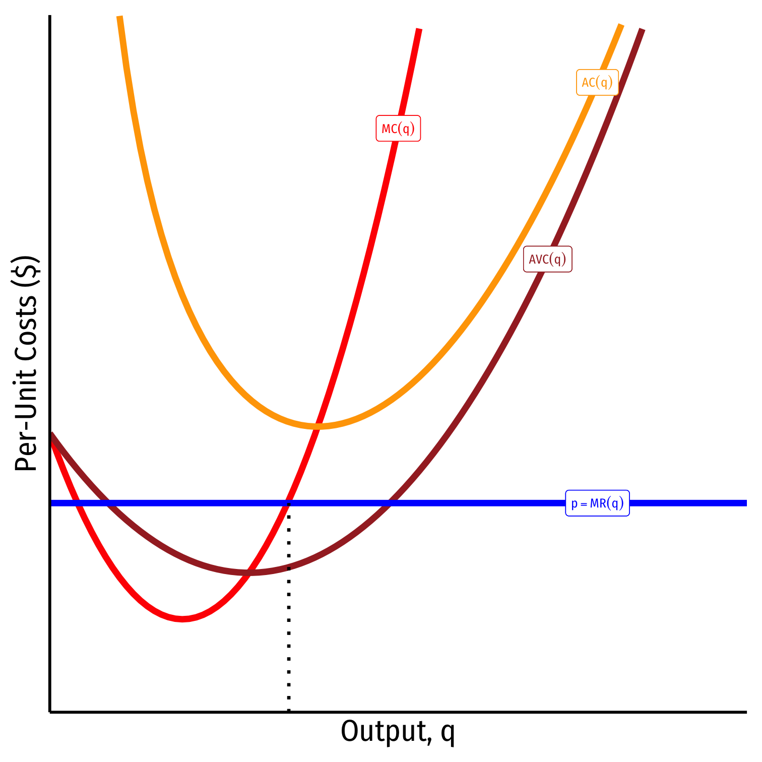
# 2.5 — Short Run Profit Maximization

## ECON 306 • Microeconomic Analysis • Spring 2023

### Ryan Safner Associate Professor of Economics <a href="mailto:safner@hood.edu">safner@hood.edu</a> <a href="https://github.com/ryansafner/microS23">ryansafner/microS23</a> <a href="https://microS23.classes.ryansafner.com"> microS23.classes.ryansafner.com</a>

---

# Outline

### [Revenues](#3)
### [Profits](#16)
### [Comparative Statics](#26)
### [Calculating Profit](#30)
### [Short-Run Shut-Down Decisions](#42)
### [The Firm's Short-Run Supply Decision](#53)

---

# Revenues

---

# Revenues for Firms in *Competitive* Industries I

.pull-left[
<img src="2.5-slides_files/figure-html/unnamed-chunk-1-1.png" width="504" style="display: block; margin: auto;" />
]

.pull-right[
<img src="2.5-slides_files/figure-html/industry-graph-1.png" width="504" style="display: block; margin: auto;" />
]

---

# Revenues for Firms in *Competitive* Industries I

.pull-left[
<img src="2.5-slides_files/figure-html/unnamed-chunk-2-1.png" width="504" style="display: block; margin: auto;" />
]

.pull-right[
<img src="2.5-slides_files/figure-html/unnamed-chunk-3-1.png" width="504" style="display: block; margin: auto;" />
]

- .blue[Demand for a firm’s product] is **perfectly elastic** at the market price

- Where did the .red[supply curve] come from? You’ll know today

---

# Revenues for Firms in *Competitive* Industries II

.pull-left[
<img src="2.5-slides_files/figure-html/unnamed-chunk-4-1.png" width="504" style="display: block; margin: auto;" />
]

- .hi[Total Revenue] `$R(q)=pq$`
]

---

# Average and Marginal Revenues

- .hi[Average Revenue]: revenue per unit of output
`$$AR(q)=\frac{R}{q}$$`
  - `$AR(q)$` is **by definition** equal to the price! (Why?)

- .hi[Marginal Revenue]: change in revenues for each additional unit of output sold:
`$$\color{#e64173}{MR(q) = \frac{\Delta R(q)}{\Delta q}}$$`
  - Calculus: first derivative of the revenues function
  - .hi-purple[For a .ul[*competitive*] firm (only), MR(q) = p, i.e. the price!]

---

# Average and Marginal Revenues: Example

.bg-washed-green.b--dark-green.ba.bw2.br3.shadow-5.ph4.mt5[
.green[**Example**]: A firm sells bushels of wheat in a very competitive market. The current market price is .blue[$10/bushel].
]

For the 1st bushel sold:

- What is the total revenue?

- What is the average revenue?

]

- What is the total revenue?

- What is the average revenue?

- What is the marginal revenue?
]

---

# Total Revenue, Example: Visualized

.quitesmall[
| `$q$` | `$R(q)$` |
|----:|-------:|
| `$0$` | `$0$` |
| `$1$` | `$10$` |
| `$2$` | `$20$` |
| `$3$` | `$30$` |
| `$4$` | `$40$` |
| `$5$` | `$50$` |
| `$6$` | `$60$` |
| `$7$` | `$70$` |
| `$8$` | `$80$` |
| `$9$` | `$90$` |
| `$10$` | `$100$` |

]
]

<img src="2.5-slides_files/figure-html/unnamed-chunk-5-1.png" width="504" style="display: block; margin: auto;" />
]

---

# Average and Marginal Revenue, Example: Visualized

| `$q$` | `$R(q)$` | `$AR(q)$` | `$MR(q)$` |
|----:|-------:|--------:|--------:|
| `$0$` | `$0$` | `$-$` | `$-$` |
| `$1$` | `$10$` | `$10$` | `$10$` |
| `$2$` | `$20$` | `$10$` | `$10$` |
| `$3$` | `$30$` | `$10$` | `$10$` |
| `$4$` | `$40$` | `$10$` | `$10$` |
| `$5$` | `$50$` | `$10$` | `$10$` |
| `$6$` | `$60$` | `$10$` | `$10$` |
| `$7$` | `$70$` | `$10$` | `$10$` |
| `$8$` | `$80$` | `$10$` | `$10$` |
| `$9$` | `$90$` | `$10$` | `$10$` |
| `$10$` | `$100$` | `$10$` | `$10$` |

]
]

<img src="2.5-slides_files/figure-html/unnamed-chunk-6-1.png" width="504" style="display: block; margin: auto;" />
]

---

# Profits

---

# Recall: The Firm's Two Problems

1. **Choose:** .hi-blue[ < output >]

2. **In order to maximize:** .hi-green[< profits >]

2nd Stage: .hi[firm's cost minimization problem]:

1. **Choose:** .hi-blue[ < inputs >]

2. **In order to _minimize_:** .hi-green[< cost >]

3. **Subject to:** .hi-red[< producing the optimal output >]

- Minimizing costs `$\iff$` maximizing profits
]
]

---

# Visualizing Total Profit As `$R(q)-C(q)$`

- `$\color{green}{\pi(q)}=\color{blue}{R(q)}-\color{red}{C(q)}$`

]

<img src="2.5-slides_files/figure-html/unnamed-chunk-7-1.png" width="504" style="display: block; margin: auto;" />
]

---

# Visualizing Total Profit As `$R(q)-C(q)$`

- `$\color{green}{\pi(q)}=\color{blue}{R(q)}-\color{red}{C(q)}$`

]

<img src="2.5-slides_files/figure-html/unnamed-chunk-8-1.png" width="504" style="display: block; margin: auto;" />
]

---

# Visualizing Total Profit As `$R(q)-C(q)$`

- `$\color{green}{\pi(q)}=\color{blue}{R(q)}-\color{red}{C(q)}$`

- Graph: find `$q^*$` to max `$\pi \implies q^*$` where max distance between `$R(q)$` and `$C(q)$`

]

<img src="2.5-slides_files/figure-html/unnamed-chunk-9-1.png" width="504" style="display: block; margin: auto;" />
]

---

# Visualizing Total Profit As `$R(q)-C(q)$`

- `$\color{green}{\pi(q)}=\color{blue}{R(q)}-\color{red}{C(q)}$`

- Graph: find `$q^*$` to max `$\pi \implies q^*$` where max distance between `$R(q)$` and `$C(q)$`

- Slopes must be equal:
`$$\color{blue}{MR(q)}=\color{red}{MC(q)}$$`

]

<img src="2.5-slides_files/figure-html/unnamed-chunk-10-1.png" width="504" style="display: block; margin: auto;" />
]

---

# Visualizing Total Profit As `$R(q)-C(q)$`

- `$\color{green}{\pi(q)}=\color{blue}{R(q)}-\color{red}{C(q)}$`

- Graph: find `$q^*$` to max `$\pi \implies q^*$` where max distance between `$R(q)$` and `$C(q)$`

- Slopes must be equal:
`$$\color{blue}{MR(q)}=\color{red}{MC(q)}$$`

.smallest[
- At `$q^*=5$`:
  - `$\color{blue}{R(q)=50}$`
  - `$\color{red}{C(q)=40}$`
  - `$\color{green}{\pi(q)=10}$`
]
]

<img src="2.5-slides_files/figure-html/unnamed-chunk-11-1.png" width="504" style="display: block; margin: auto;" />
]

---

# Visualizing Profit Per Unit As `$MR(q)$` and `$MC(q)$`

- At low output `$q<q^*$`, can increase `$\pi$` by producing *more*: `$\color{blue}{MR(q)}>\color{red}{MC(q)}$`

]

<img src="2.5-slides_files/figure-html/unnamed-chunk-12-1.png" width="504" style="display: block; margin: auto;" />
]

---

# Visualizing Profit Per Unit As `$MR(q)$` and `$MC(q)$`

- At high output `$q>q^*$`, can increase `$\pi$` by producing *less*: `$\color{blue}{MR(q)}<\color{red}{MC(q)}$`

]

<img src="2.5-slides_files/figure-html/unnamed-chunk-13-1.png" width="504" style="display: block; margin: auto;" />
]

---

# Visualizing Profit Per Unit As `$MR(q)$` and `$MC(q)$`

- `$\pi$` is *maximized* where `$\color{blue}{MR(q)}=\color{red}{MC(q)}$`

]

<img src="2.5-slides_files/figure-html/unnamed-chunk-14-1.png" width="504" style="display: block; margin: auto;" />
]

---

# Comparative Statics

---

# If Market Price Changes I

- Suppose the market price **increases**

- Firm (always setting .blue[MR]=.red[MC]) will respond by **producing more**

]

<img src="2.5-slides_files/figure-html/unnamed-chunk-15-1.png" width="504" style="display: block; margin: auto;" />
]

---

# If Market Price Changes II

- Suppose the market price **decreases**

- Firm (always setting .blue[MR]=.red[MC]) will respond by **producing less**

]

<img src="2.5-slides_files/figure-html/unnamed-chunk-16-1.png" width="504" style="display: block; margin: auto;" />
]

---

# The Firm’s Supply Curve

- .hi-purple[The firm’s marginal cost curve is its supply curve].magenta[‡]
`$$\color{red}{p=MC(q)}$$`
 - How it will supply the optimal amount of output in response to the market price
 - .hi-purple[Firm always sets its price equal to its marginal cost]

]

<img src="2.5-slides_files/figure-html/unnamed-chunk-17-1.png" width="504" style="display: block; margin: auto;" />
]

---

# Calculating Profit

---

# Calculating (Average) Profit as AR(q)-AC(q)

- Profit is 
`$$\pi(q)=R(q)-C(q)$$`

]

<img src="2.5-slides_files/figure-html/unnamed-chunk-18-1.png" width="504" style="display: block; margin: auto;" />
]

---

# Calculating (Average) Profit as AR(q)-AC(q)

- Profit is 
`$$\pi(q)=R(q)-C(q)$$`

- Profit per unit can be calculated as:
`$$\begin{align*}
\frac{\pi(q)}{q}&=\color{blue}{AR(q)}-\color{orange}{AC(q)}\\
&=\color{blue}{p}-\color{orange}{AC(q)}\\
\end{align*}$$`

]

<img src="2.5-slides_files/figure-html/unnamed-chunk-19-1.png" width="504" style="display: block; margin: auto;" />
]

---
# Calculating (Average) Profit as AR(q)-AC(q)

- Profit is 
`$$\pi(q)=R(q)-C(q)$$`

- Profit per unit can be calculated as:
`$$\begin{align*}
\frac{\pi(q)}{q}&=\color{blue}{AR(q)}-\color{orange}{AC(q)}\\
&=\color{blue}{p}-\color{orange}{AC(q)}\\
\end{align*}$$`

- Multiply by `$q$` to get total profit:
`$$\pi(q)=q\left[\color{blue}{p}-\color{orange}{AC(q)} \right]$$`

]

<img src="2.5-slides_files/figure-html/unnamed-chunk-20-1.png" width="504" style="display: block; margin: auto;" />
]

---

# Calculating (Average) Profit as AR(q)-AC(q)

- At market price of .blue[p* = $10]

- At q* = 5 (per unit):

- At q* = 5 (totals):

]

<img src="2.5-slides_files/figure-html/unnamed-chunk-21-1.png" width="504" style="display: block; margin: auto;" />
]

---

# Calculating (Average) Profit as AR(q)-AC(q)

- At market price of .blue[p* = $10]

- At q* = 5 (per unit):
  - .blue[AR(5) = $10/unit]

- At q* = 5 (totals):
  - .blue[R(5) = $50]
]

<img src="2.5-slides_files/figure-html/unnamed-chunk-22-1.png" width="504" style="display: block; margin: auto;" />
]

---

# Calculating (Average) Profit as AR(q)-AC(q)

- At market price of .blue[p* = $10]

- At q* = 5 (per unit):
  - .blue[AR(5) = $10/unit]
  - .orange[AC(5) = $7/unit]

- At q* = 5 (totals):
  - .blue[R(5) = $50]
  - .red[C(5) = $35]
]

<img src="2.5-slides_files/figure-html/unnamed-chunk-23-1.png" width="504" style="display: block; margin: auto;" />
]

---

# Calculating (Average) Profit as AR(q)-AC(q)

- At market price of .blue[p* = $10]

- At q* = 5 (per unit):
  - .blue[AR(5) = $10/unit]
  - .orange[AC(5) = $7/unit]
  - .green[A`\$\pi\$`(5) = $3/unit]

- At q* = 5 (totals):
  - .blue[R(5) = $50]
  - .red[C(5) = $35]
  - .green[`\$\pi\$` = $15]
]

<img src="2.5-slides_files/figure-html/unnamed-chunk-24-1.png" width="504" style="display: block; margin: auto;" />
]

---

# Calculating (Average) Profit as AR(q)-AC(q)

- At market price of .blue[p* = $2]

- At q* = 1 (per unit):

- At q* = 1 (totals):

]

<img src="2.5-slides_files/figure-html/unnamed-chunk-25-1.png" width="504" style="display: block; margin: auto;" />
]

---

# Calculating (Average) Profit as AR(q)-AC(q)

- At market price of .blue[p* = $2]

- At q* = 1 (per unit):
  - .blue[AR(1) = $2/unit]

- At q* = 1 (totals):
  - .blue[R(1) = $2]
]

<img src="2.5-slides_files/figure-html/unnamed-chunk-26-1.png" width="504" style="display: block; margin: auto;" />
]

---

# Calculating (Average) Profit as AR(q)-AC(q)

- At market price of .blue[p* = $2]

- At q* = 1 (per unit):
  - .blue[AR(1) = $2/unit]
  - .orange[AC(1) = $10/unit]

- At q* = 1 (totals):
  - .blue[R(1) = $2]
  - .red[C(1) = $10]

]

<img src="2.5-slides_files/figure-html/unnamed-chunk-27-1.png" width="504" style="display: block; margin: auto;" />
]

---

# Calculating (Average) Profit as AR(q)-AC(q)

- At market price of .blue[p* = $2]

- At q* = 1 (per unit):
  - .blue[AR(1) = $2/unit]
  - .orange[AC(1) = $10/unit]
  - .green[A`\$\pi\$`(1) = -$8/unit]

- At q* = 1 (totals):
  - .blue[R(1) = $2]
  - .red[C(1) = $10]
  - .green[`\$\pi\$`(1) = -$8]
]

<img src="2.5-slides_files/figure-html/unnamed-chunk-28-1.png" width="504" style="display: block; margin: auto;" />
]

---