3.2 — Market Competition & Surpluses
ECON 306 • Microeconomic Analysis • Spring 2023
Ryan Safner
Associate Professor of Economics
safner@hood.edu
ryansafner/microS23
microS23.classes.ryansafner.com
The Algebra of Calculating Equilibrium
The Algebra of Calculating Equilibrium
Simple algebra to find equilibrium prices and quantities if we know supply and demand functions
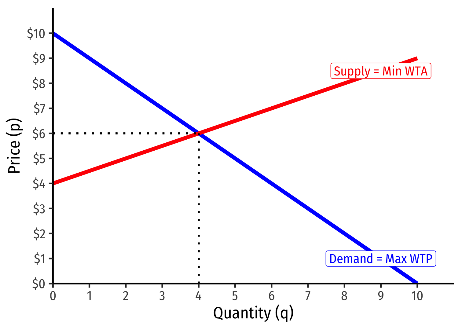
Remember, supply and demand are each mathematical functions relating price to quantity:
- Demand: qD=10−p
- Supply: qS=2p−8
We know at equilibrium: qD=qS
Calculating Equilibrium: Another Example
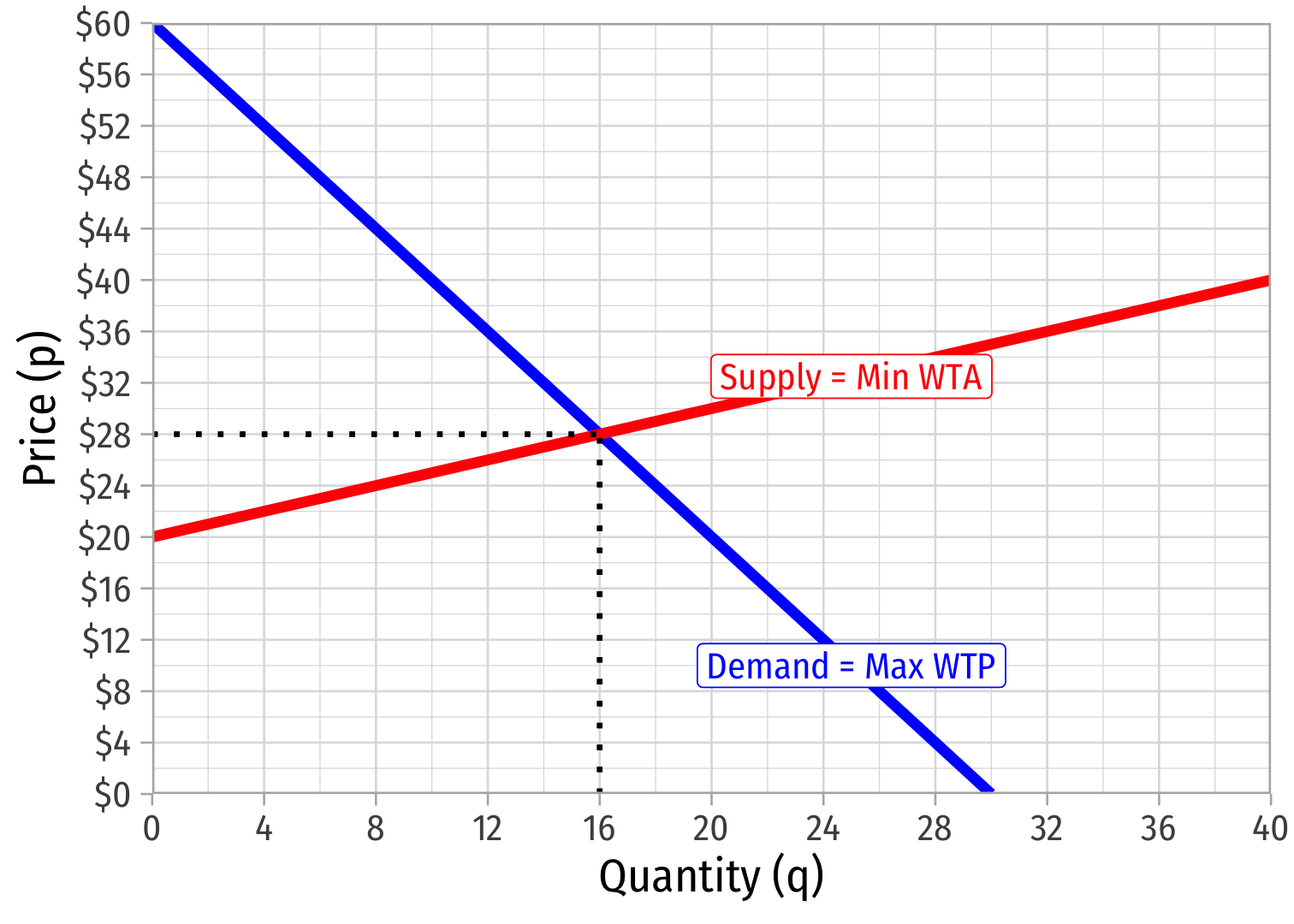
Example: Let the supply and demand functions for a market be:
qD=30−0.5pqS=2p−40
Find equilibrium quantity and price (q⋆,p⋆).
Sketch a rough graph.
Calculating Equilibrium: Another Example
Example: Let the supply and demand functions for a market be:
qD=30−0.5pqS=2p−40
Find equilibrium quantity and price (q⋆,p⋆).
Sketch a rough graph.
Price Competition in Markets
Price Competition in Markets I
Markets allocate resources based on individuals’ reservation prices:
- Buyers’ max. willingness to pay
- Sellers’ min. willingness to accept
Goods flow to those who value them the highest and away from those who value them the lowest
Price Competition in Markets I
Markets allocate resources based on individuals’ reservation prices:
- Buyers’ max. willingness to pay
- Sellers’ min. willingness to accept
Goods flow to those who value them the highest and away from those who value them the lowest

Price Competition in Markets II
It might look like it, but competition in markets is NOT between buyers vs. sellers!
In markets:
- buyers compete with other buyers &
- sellers compete with other sellers

Price Competition Between Buyers
Buyers want to pay the lowest price to buy a good
But they face competition from other buyers over the same scarce goods
Buyers attempt to raise their bids above others' reservation prices to obtain the goods

Price Competition Between Sellers
Sellers want to get the highest price for a good they sell
But they face competition from other sellers over the same potential customers
Sellers attempt to lower their asking prices below others' reservation prices to sell their goods

An Example

Imagine a small public horse market
3 people, A, B, and C each own 1 horse
3 people, D, E, and F each are potentially interested in buying a horse
This example is based on Eugen von Bohm-Bawerk’s famous example in Capital and Interest (1884)
An Example
| Person | Reservation Price |
|---|---|
| A | Minimum WTA: $400 |
| B | Minimum WTA: $500 |
| C | Minimum WTA: $600 |
| D | Maximum WTP: $600 |
| E | Maximum WTP: $500 |
| F | Maximum WTP: $400 |
Imagine a small public horse market
3 people, A, B, and C each own 1 horse
3 people, D, E, and F each are potentially interested in buying a horse
An Example
| Person | Reservation Price |
|---|---|
| A | Minimum WTA: $400 |
| B | Minimum WTA: $500 |
| C | Minimum WTA: $600 |
| D | Maximum WTP: $600 |
| E | Maximum WTP: $500 |
| F | Maximum WTP: $400 |
Price: $400
Suppose Buyer F announces she will pay $400 for a horse
Only Seller A is willing to sell at $400
Buyers D, E, and F are willing to buy at $400
- D and E are willing to pay more than F to obtain the 1 horse
- A shortage: 3 buyers for 1 seller!
- They raise their bids above $400 to attract sellers
An Example
| Person | Reservation Price |
|---|---|
| A | Minimum WTA: $400 |
| B | Minimum WTA: $500 |
| C | Minimum WTA: $600 |
| D | Maximum WTP: $600 |
| E | Maximum WTP: $500 |
| F | Maximum WTP: $400 |
Price: $600
Suppose Seller C announces he will sell his horse for $600
Only Buyer D is willing to buy at $600
Sellers A, B, and C are willing to sell at $600
- A and B are willing to accept less than C to sell their horses
- A surplus: 3 sellers for 1 buyer!
- They lower their asks below $600 to attract buyers
An Example
| Person | Reservation Price |
|---|---|
| A | Minimum WTA: $400 |
| B | Minimum WTA: $500 |
| C | Minimum WTA: $600 |
| D | Maximum WTP: $600 |
| E | Maximum WTP: $500 |
| F | Maximum WTP: $400 |
Price: $500
If the market price reaches $500 (through bids and asks changing):
Sellers A and B sell their horses for $500 each
- Buyers D and E buy them at $500 each
An Example: Price is Determined at the Margin
| Person | Reservation Price |
|---|---|
| A | Minimum WTA: $400 |
| B | Minimum WTA: $500 |
| C | Minimum WTA: $600 |
| D | Maximum WTP: $600 |
| E | Maximum WTP: $500 |
| F | Maximum WTP: $400 |
Price: $500
At $500, B and E are the “marginal” buyer and seller, the “last” ones that just got off the fence to exchange in the market
- B has WTA just low enough to sell
- E has WTP just high enough to buy
The marginal pair actually are the ones that “set” the market price!
An Example: Price is Determined at the Margin
| Person | Reservation Price |
|---|---|
| A | Minimum WTA: $400 |
| B | Minimum WTA: $500 |
| C | Minimum WTA: $600 |
| D | Maximum WTP: $600 |
| E | Maximum WTP: $500 |
| F | Maximum WTP: $400 |
Price: $500
Notice the most possible exchanges take place at a market price of $500
- 2 horses get exchanged
Any price above or below $500, only 1 horse would get exchanged
- Also, at least one other buyer or seller would raise/lower their bid/ask
An Example: Excluded Parties
| Person | Reservation Price |
|---|---|
| A | Minimum WTA: $400 |
| B | Minimum WTA: $500 |
| C | Minimum WTA: $600 |
| D | Maximum WTP: $600 |
| E | Maximum WTP: $500 |
| F | Maximum WTP: $400 |
Price: $500
- At $500, C and F are the “excluded” buyers and sellers
- C has WTA too high to sell
- F has WTP too low to buy
An Example: Inframarginal Parties
| Person | Reservation Price |
|---|---|
| A | Minimum WTA: $400 |
| B | Minimum WTA: $500 |
| C | Minimum WTA: $600 |
| D | Maximum WTP: $600 |
| E | Maximum WTP: $500 |
| F | Maximum WTP: $400 |
Price: $500
At $500, A and D are the “inframarginal” buyers and sellers
- A has WTA lower than market price, earns extra $100 surplus from exchange
- D has WTP higher than market price, earns extra $100 surplus from exchange
These buyers and sellers benefit the most from exchange
Economic Surplus
Market-Clearing Prices
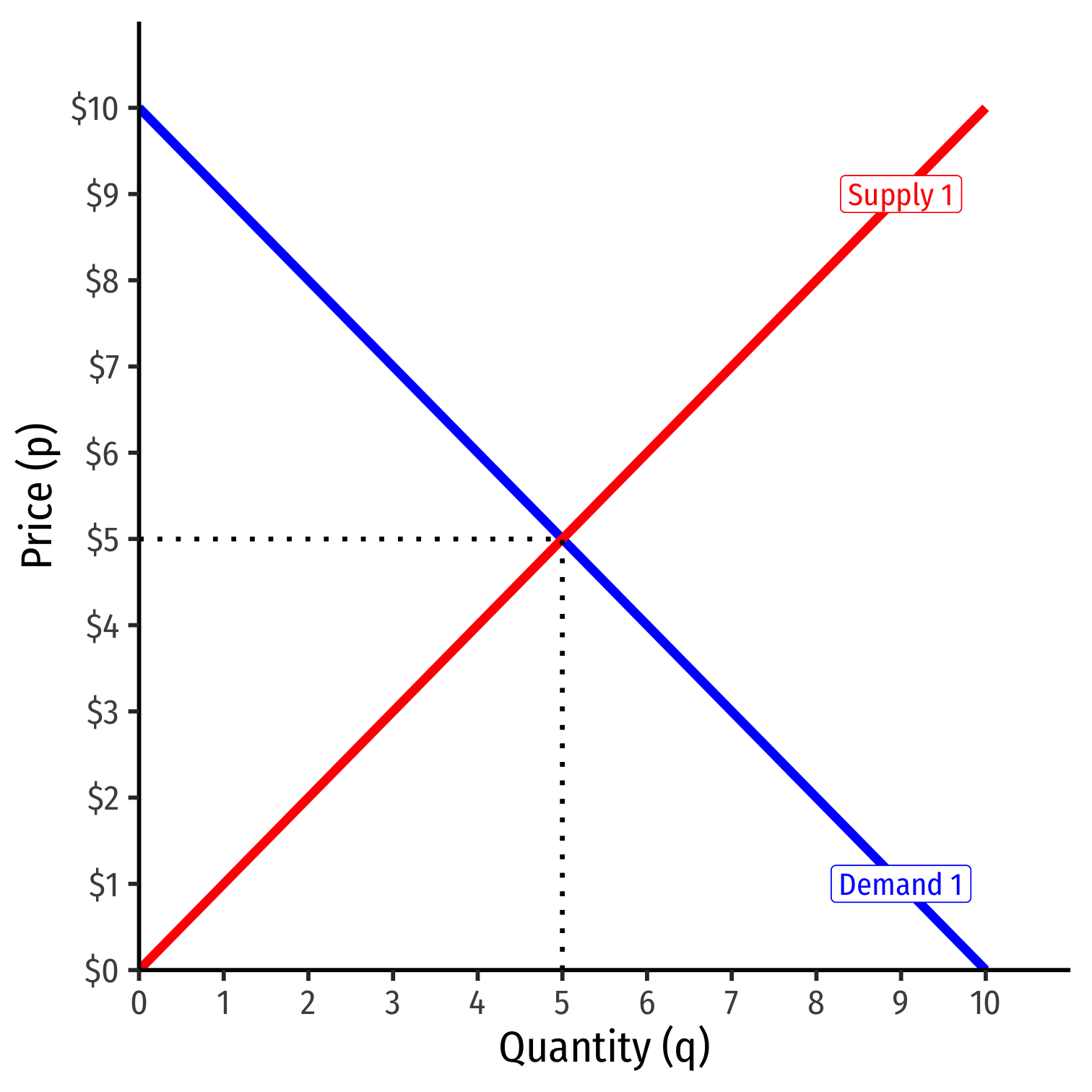
- Supply and demand set the market-clearing price for all units exchanged (bought and sold)
Consumer Surplus I
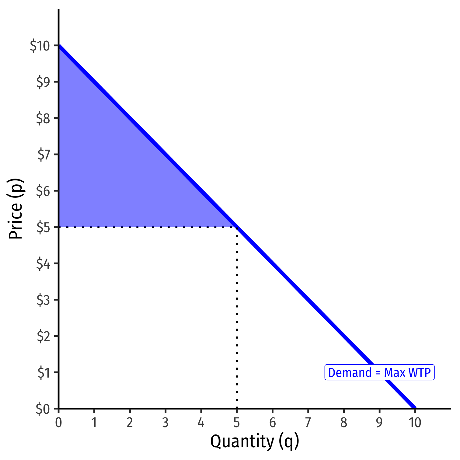
Demand function measures how much you would hypothetically be willing to pay for various quantities
- "reservation price"
You often actually pay (the market-clearing price, p∗) a lot less than your reservation price
The difference is consumer surplus
CS=WTP−p∗

Consumer Surplus II
CS=12bhCS=12(5−0)($10−$5)CS=$12.50
Consumer Surplus III
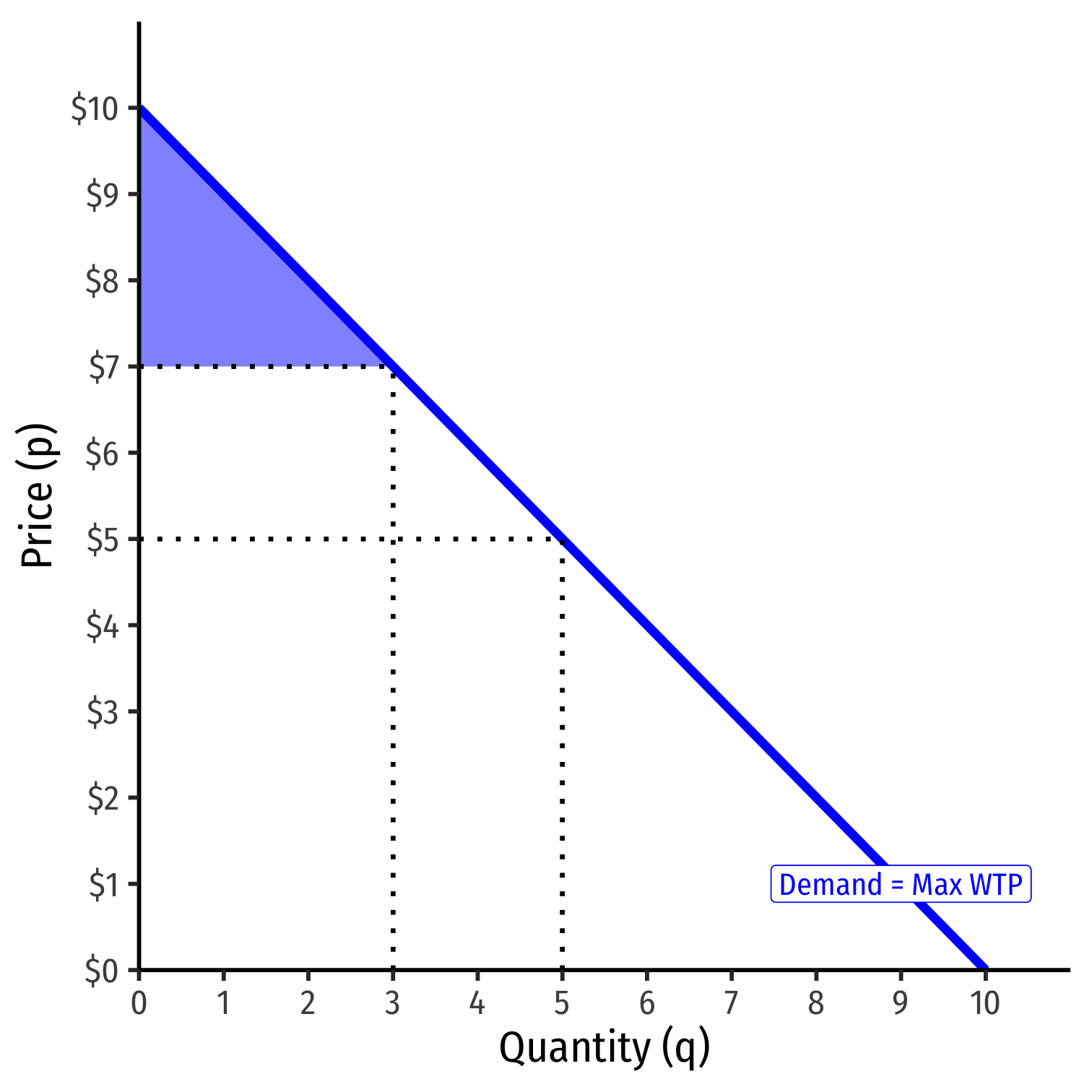
- An increase in market price reduces consumer surplus
CS′=12bhCS′=12(3−0)($10−$7)CS′=$4.50
Consumer Surplus IV
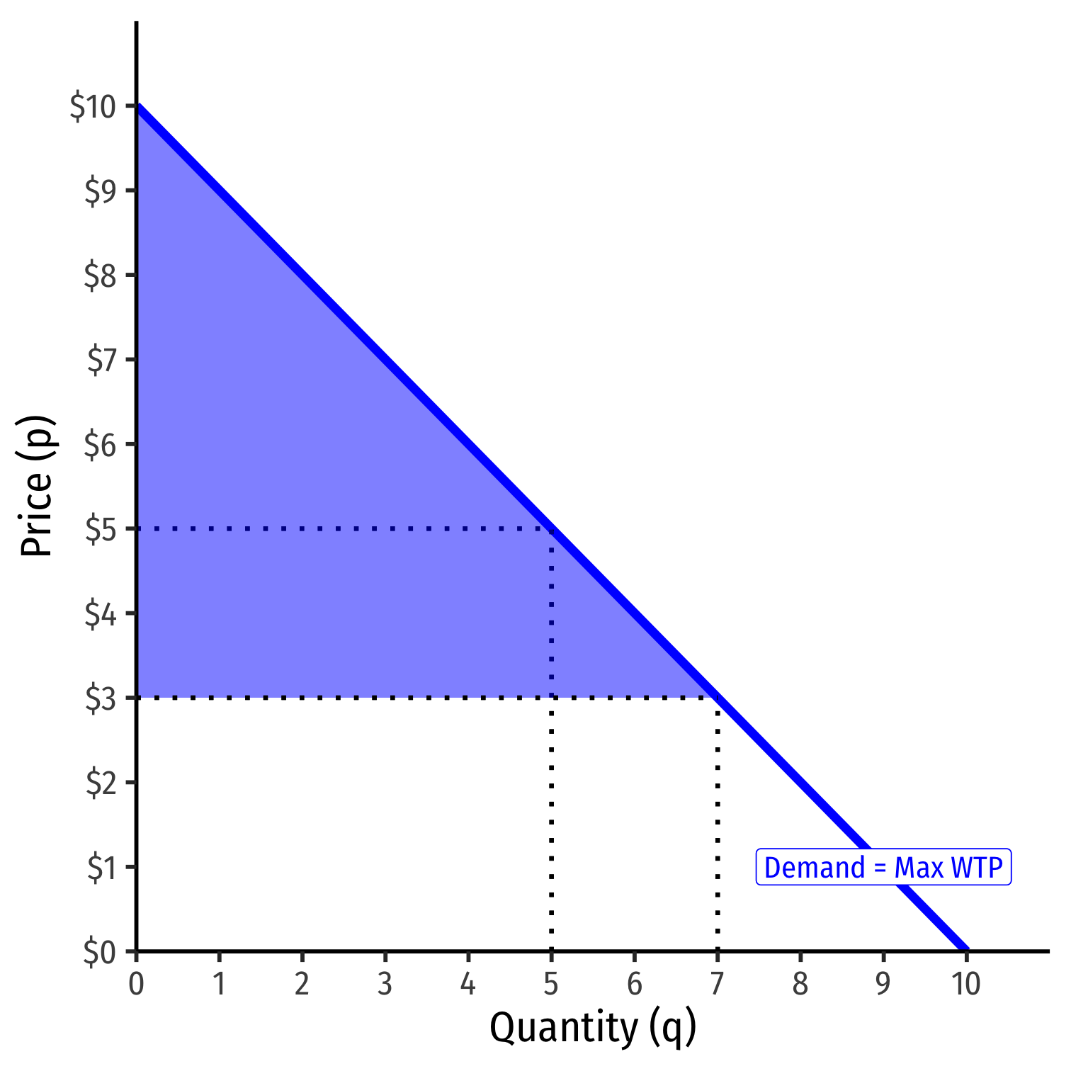
- An decrease in market price increases consumer surplus
CS′=12bhCS′=12(7−0)($10−$3)CS′=$24.50
Consumer Surplus V
- A relatively inelastic demand curve generates more consumer surplus
CS=12(5−0)($10−$5)CS=$12.50

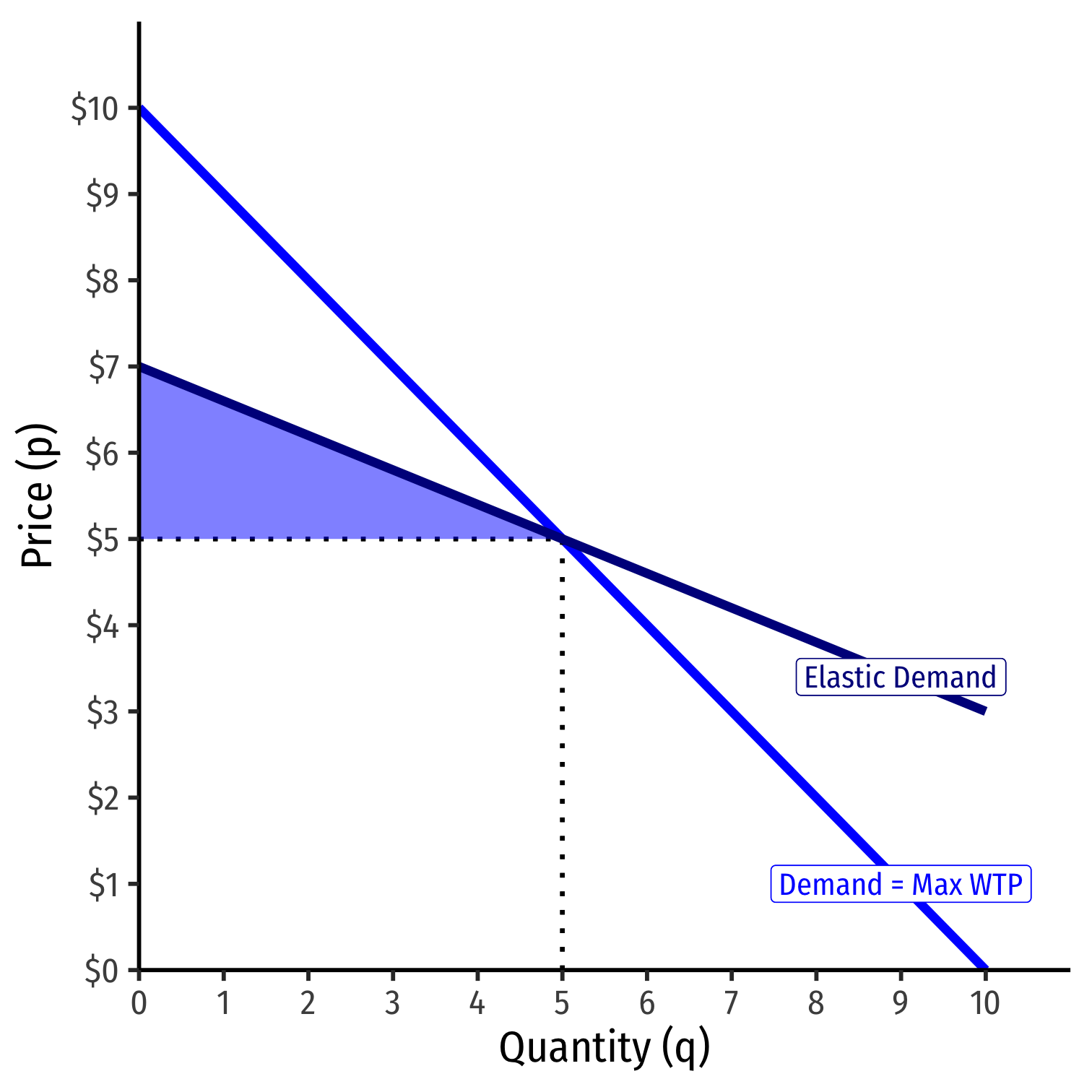
Consumer Surplus V
- A relatively inelastic demand curve generates more consumer surplus
CS=12(5−0)($10−$5)CS=$12.50
- A relatively elastic demand curve generates less consumer surplus
CS=12(5−0)($7−$5)CS=$5.00
Producer Surplus I
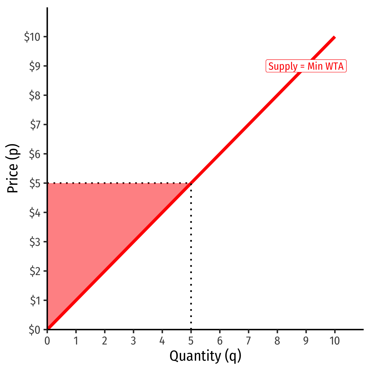
Supply function measures how much you would hypothetically be willing to accept to sell various quantities
- "reservation price"
You often actually receive (the market-clearing price, p∗) a lot more than your reservation price
The difference is producer surplus
PS=p∗−WTA
Producer Surplus II
PS=12bhPS=12(5−0)($5−$0)PS=$12.50

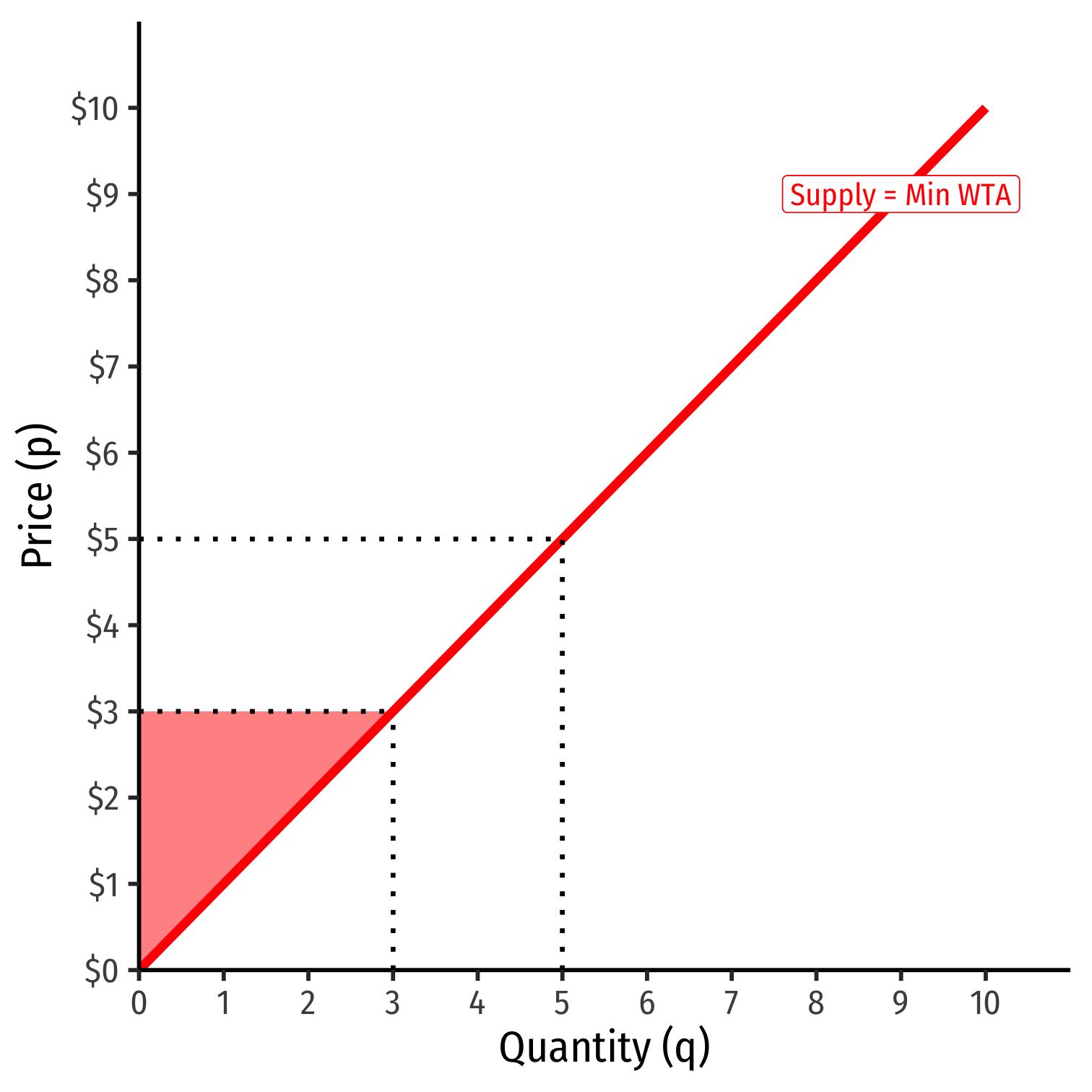
Producer Surplus III
- An increase in market price increases producer surplus
PS′=12bhPS′=12(7−0)($7−$0)PS′=$24.50
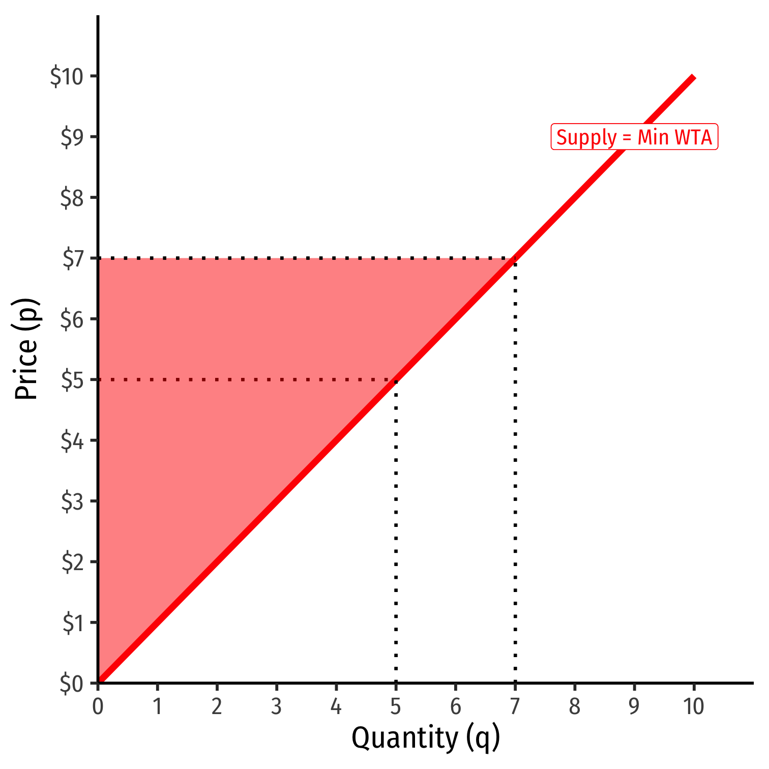
Producer Surplus IV
- An decrease in market price decreases producer surplus
PS′=12bhPS′=12(3−0)($3−$0)PS′=$4.50
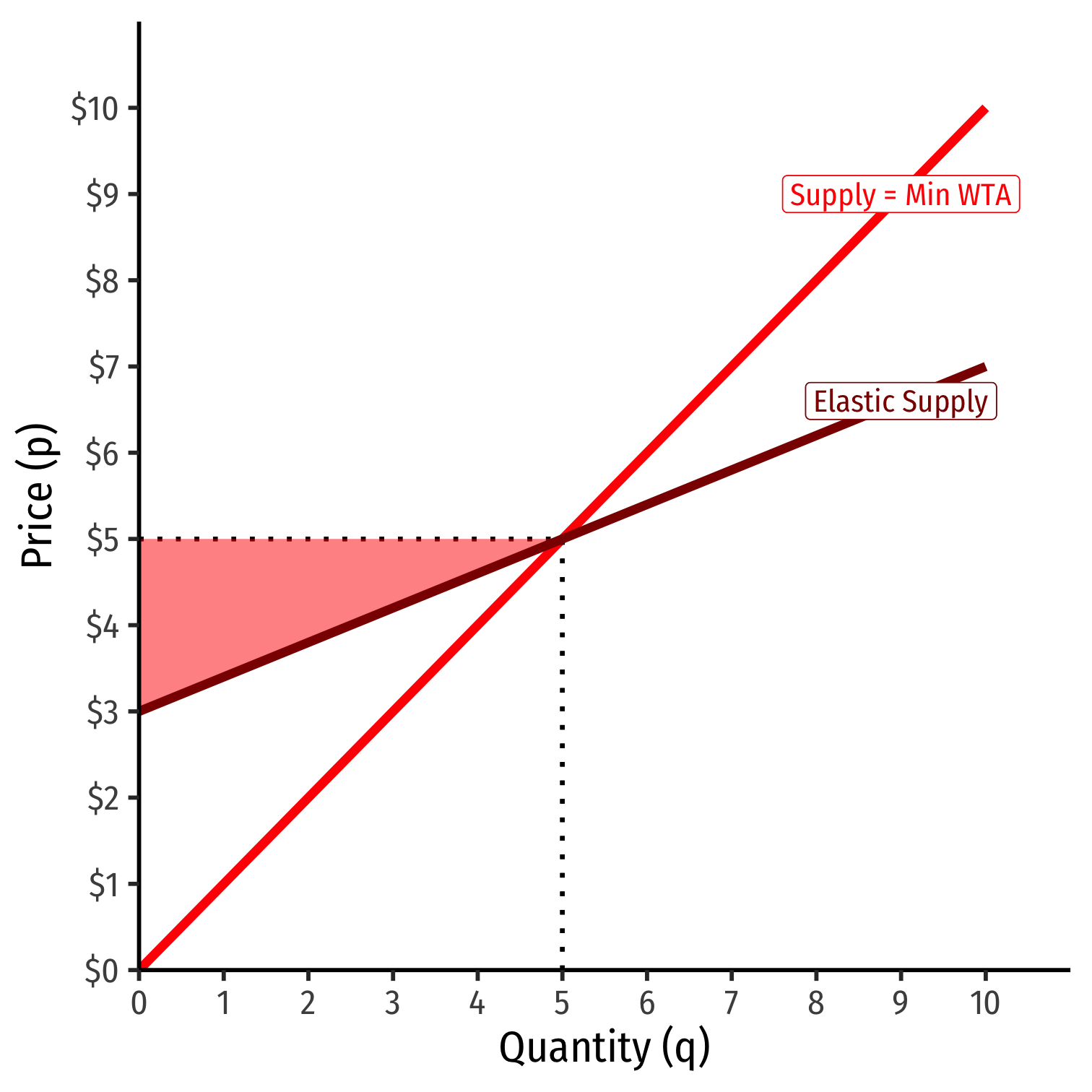
Producer Surplus V
- A relatively inelastic supply curve generates more producer surplus
PS=12(5−0)($5−$0)PS=$12.50

Producer Surplus V
- A relatively inelastic supply curve generates more producer surplus
PS=12(5−0)($5−$0)PS=$12.50
- A relatively elastic supply curve generates less producer surplus
PS=12(5−0)($5−$3)PS=$5.00
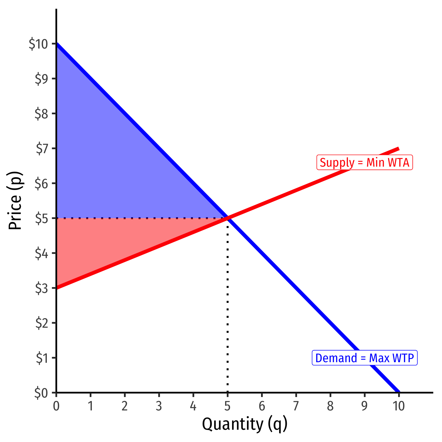
Elasticities and Surpluses I
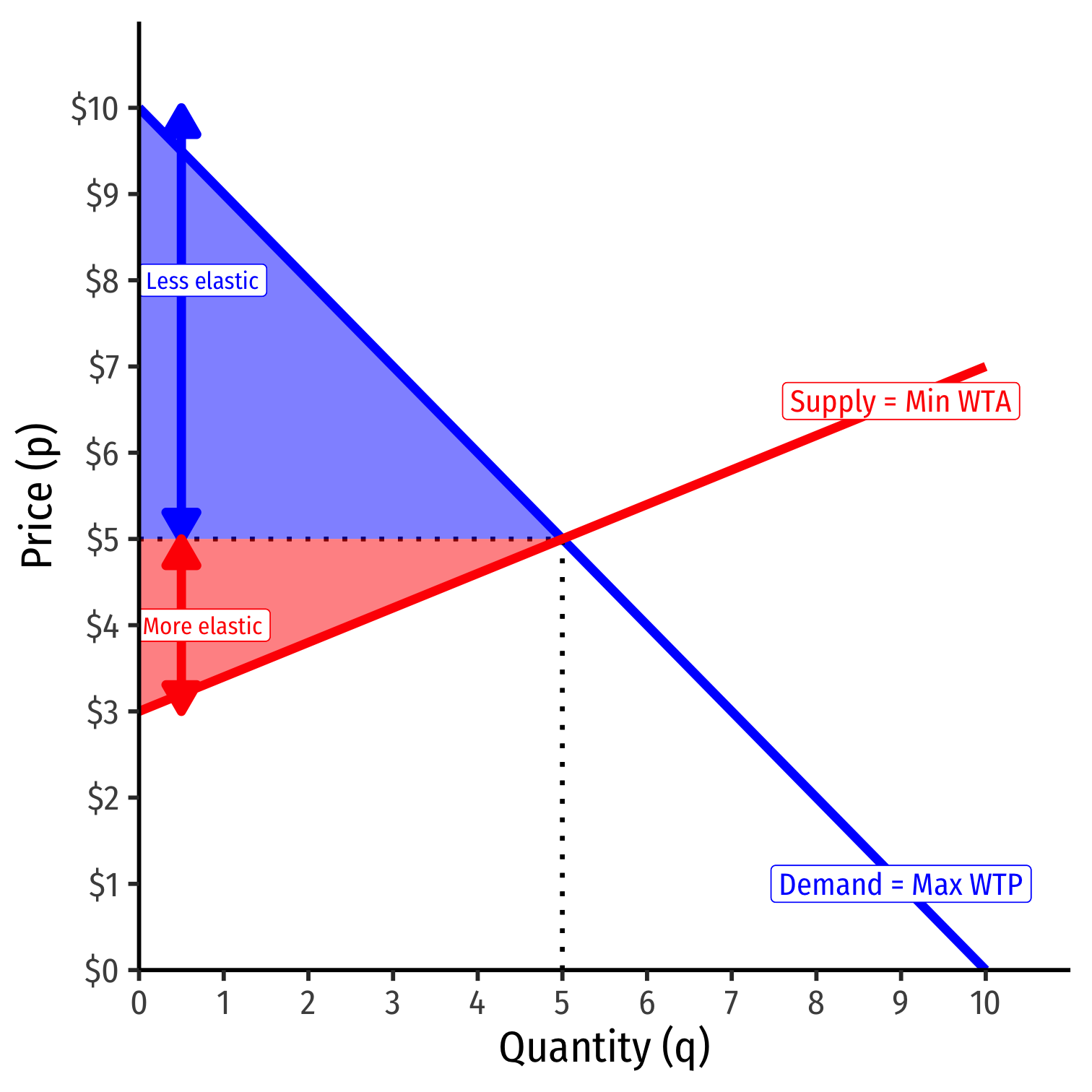
The more elastic curve at p∗ generates less surplus
- More options, easier to change choices, less benefit from any one particular exchange
The less elastic curve at p∗ generates more surplus
- Fewer options, harder to change choices, more benefit from any one particular exchange
This is important for policies such as price controls, taxes, etc.
Elasticities and Surpluses II
A good visual rule of thumb:
Compare distance between choke price and p∗ for each curve
Bigger distance ⟹ less elastic in equilibrium (and vice versa)
- ⟹ more surplus
Example
Example: Using last class's supply and demand functions:
qD=10−pqS=2p−8
Calculate the price elasticity of demand and the price elasticity of supply in equilibrium.
Calculate the consumer surplus and producer surplus. Shade each on the graph.
Who gets more surplus, consumers or producers, and why?