4.1 — Modeling Market Power
ECON 306 • Microeconomic Analysis • Spring 2023
Ryan Safner
Associate Professor of Economics
safner@hood.edu
ryansafner/microS23
microS23.classes.ryansafner.com
Market Power
Imperfect Competition

Imperfect Competition

Imperfect Competition

Imperfect Competition

Competitive Markets, Recap
For competitive markets, modeled firms as “price-takers”: so many of them selling identical products, no one could affect price p
- p⋆ must be market price, but choose q⋆ to maximize π
(Long-run) Equilibrium: Marginal cost pricing for all firms, which is allocatively efficient for society
- p=MC
- MSB=MSC
Over long-run, free entry and exit push prices to equal (average & marginal) costs and pushed economic profits to zero

Market Power

Adam Smith
1723-1790
“People of the same trade seldom meet together, even for merriment and diversion, but the conversation ends in a conspiracy against the public, or in some contrivance to raise prices. It is impossible indeed to prevent such meetings, by any law which either could be executed, or would be consistent with liberty and justice. But though the law cannot hinder people of the same trade from sometimes assembling together, it ought to do nothing to facilitate such assemblies; much less to render them necessary.” (Book I, Chapter X Part II).
Smith, Adam, 1776, An Enquiry into the Nature and Causes of the Wealth of Nations
Market Power vs. Competition
All sellers would like to raise prices and extract more revenue from consumers
Competition from other sellers (and potential entrants) drives prices to equal costs & economic profits to zero
- Firm in competitive market raising p>MC(q) would lose all of its customers!
Market power: ability to raise p>MC(q) (and not lose all customers)

Market Power vs. Competition

Adam Smith
1723-1790
“The pretence that [monopolies] are necessary for the better government of the trade, is without any foundation. The real and effectual discipline which is exercised over a [producer], is not that of his [monopoly], but that of his customers. It is the fear of losing their employment which restrains his frauds and corrects his negligence. An exclusive [monopoly] necessarily weakens the force of this discipline,” (Book I, Chapter X Part II).
Smith, Adam, 1776, An Enquiry into the Nature and Causes of the Wealth of Nations
Modeling Firms with Market Power
Firms with market power behave differently than firms in a competitive market
- Today: understanding how to model that different behavior
Start with simple assumption of a single seller: monopoly (easiest to model)
Next class:
- causes of market power
- consequences of market power

Modeling Firms with Market Power
A firm with market power is a “price-searcher”
- Firms with market power search for both (q⋆,p⋆) that maximizes π
With a monopoly model, we can safely ignore the effects that other sellers have on one firm’s behavior
- A convenient starting point
- Later, will need game theory to deal with other firms’ interactions

The Monopolist's Problem
- The monopolist’s profit maximization problem:
Choose: < output and price: (q⋆,p⋆) >
In order to maximize: < profits: π >

Marginal Revenues
Market Power and Revenues I

- Firms are constrained by relationship between quantity and price that consumers are willing to pay
Market Power and Revenues I
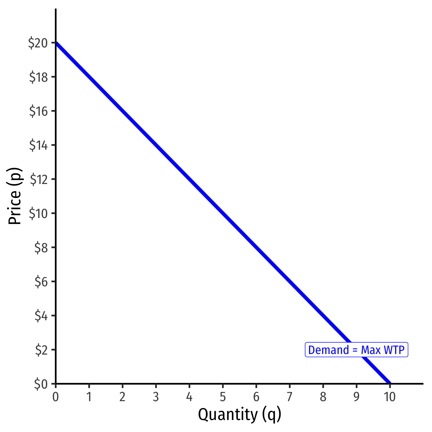
Firms are constrained by relationship between quantity and price that consumers are willing to pay
Market (inverse) demand describes maximum price consumers are willing to pay for a given quantity
Implications:
- Even a monopoly can’t set a price “as high as it wants”
- Even a monopoly can still earn losses!
Market Power and Revenues II
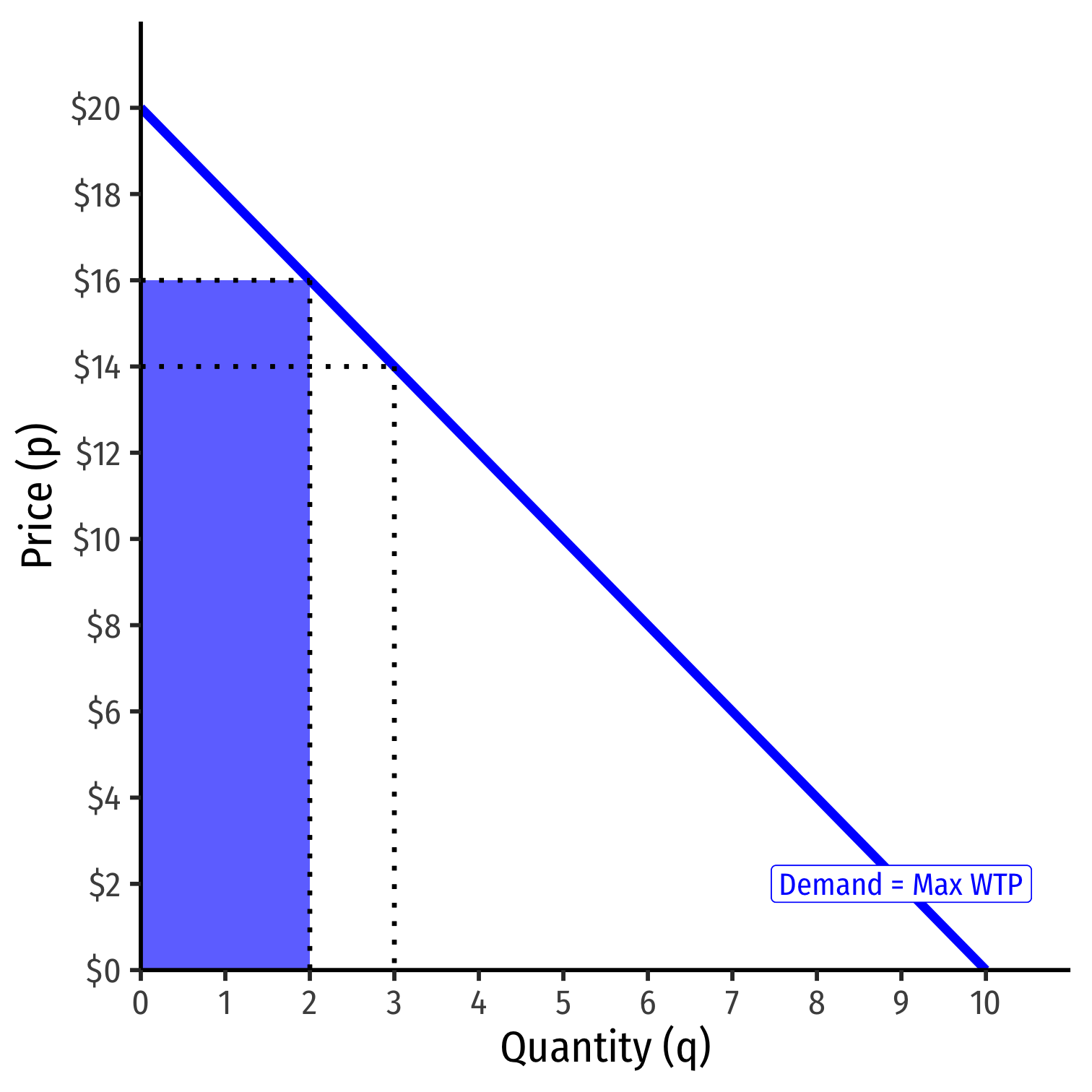
- As firm chooses to produce more q, must lower the price on all units to sell them
Market Power and Revenues II
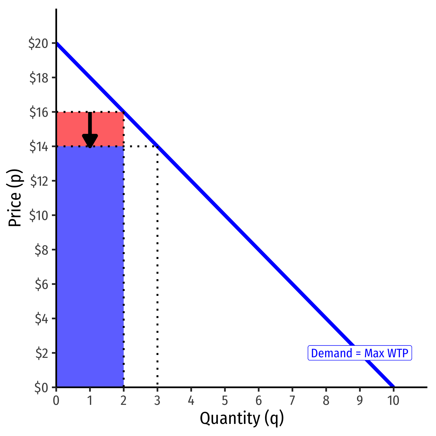
As firm chooses to produce more q, must lower the price on all units to sell them
Price effect (qΔp): lost revenue from lowering price on all sales ($2×−2)
Market Power and Revenues II

As firm chooses to produce more q, must lower the price on all units to sell them
Price effect (qΔp): lost revenue from lowering price on all sales ($2×−2)
Output effect (pΔq): gained revenue from increase in sales ($14×1)
Market Power and Revenues II
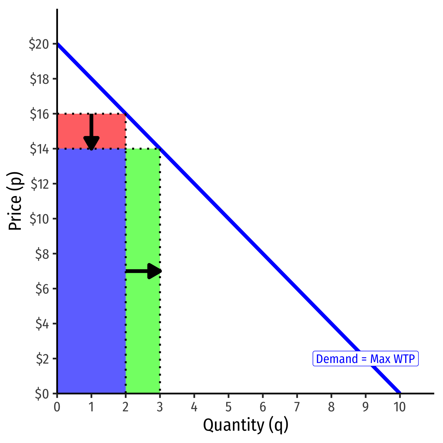
As firm chooses to produce more q, must lower the price on all units to sell them
Price effect (qΔp): lost revenue from lowering price on all sales ($2×−2)
Output effect (pΔq): gained revenue from increase in sales ($14×1)
| q | p | R(q) | Change |
|---|---|---|---|
| 2 | $16 | $32 | |
| 3 | $14 | $42 | +$10 |
Marginal Revenue I
- If a firm increases output, Δq, revenues would change by:
ΔR(q)=pΔq + qΔp
Marginal Revenue I
- If a firm increases output, Δq, revenues would change by:
ΔR(q)=pΔq + qΔp
- Output effect: increases number of units sold (Δq) times price p per unit
Marginal Revenue I
- If a firm increases output, Δq, revenues would change by:
ΔR(q)=pΔq + qΔp
Output effect: increases number of units sold (Δq) times price p per unit
Price effect: lowers price per unit (Δp) on all units sold (q)
Marginal Revenue I
- If a firm increases output, Δq, revenues would change by:
ΔR(q)=pΔq + qΔp
Output effect: increases number of units sold (Δq) times price p per unit
Price effect: lowers price per unit (Δp) on all units sold (q)
Divide both sides by Δq to get Marginal Revenue, MR(q):
ΔR(q)Δq=MR(q)=p+ΔpΔqq
- Compare: demand for a competitive firm is perfectly elastic: ΔpΔq=0, so we saw MR(q)=p!
Marginal Revenue II
- If we have a linear inverse demand function of the form
p=a+bq
- a is the choke price (intercept)
- b is the slope
Marginal Revenue II
- If we have a linear inverse demand function of the form
p=a+bq
- a is the choke price (intercept)
- b is the slope
- Marginal revenue again is defined as: MR(q)=p+ΔpΔqq
Marginal Revenue II
- If we have a linear inverse demand function of the form
p=a+bq
- a is the choke price (intercept)
- b is the slope
- Marginal revenue again is defined as: MR(q)=p+ΔpΔqq
- Recognize that ΔpΔq=(riserun) is the slope, b,
Marginal Revenue II
- If we have a linear inverse demand function of the form
p=a+bq
- a is the choke price (intercept)
- b is the slope
- Marginal revenue again is defined as: MR(q)=p+ΔpΔqq
- Recognize that ΔpΔq=(riserun) is the slope, b,
MR(q)=p+(b)qMR(q)=(a+bq)+bqMR(q)=a+2bq
Marginal Revenue III
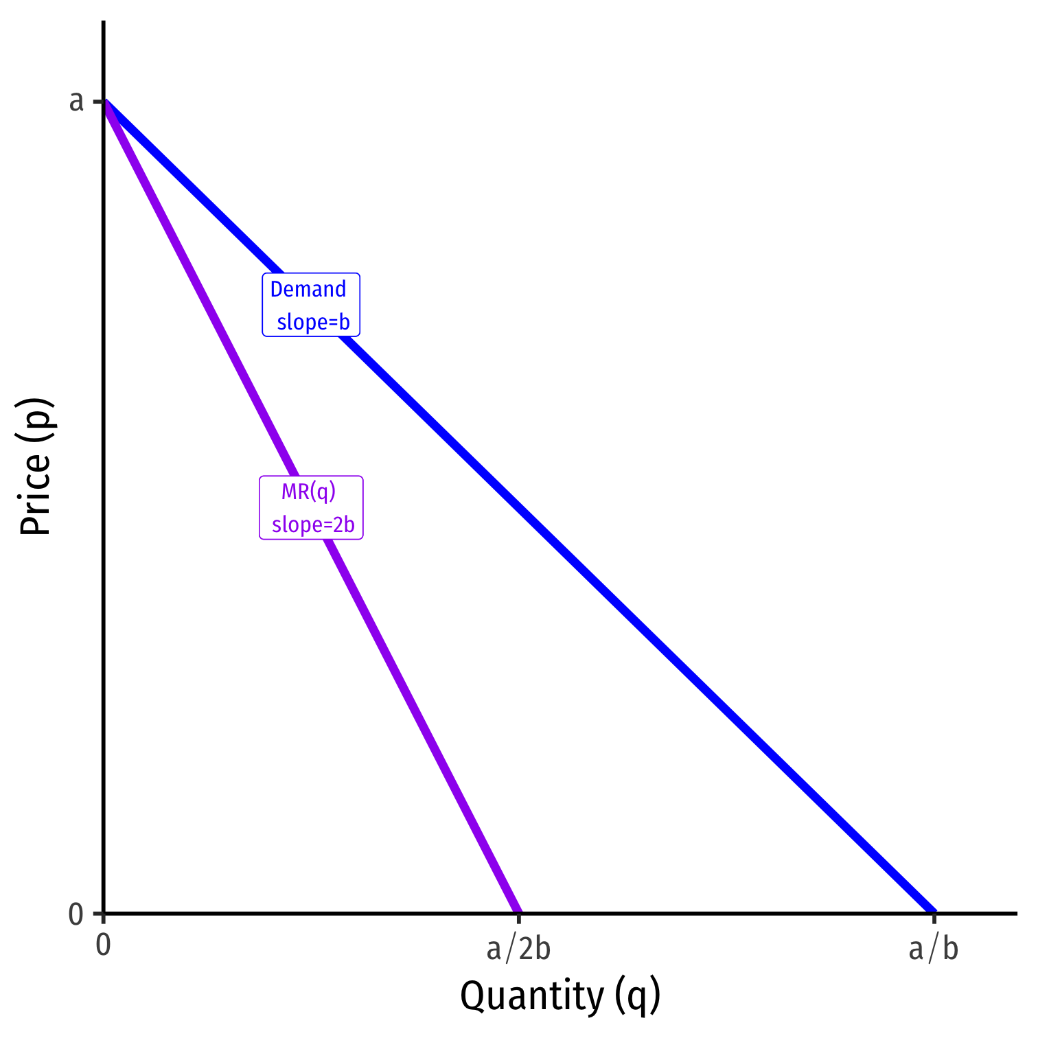
p(q)=a+bqMR(q)=a+2bq
Marginal revenue starts at same intercept as Demand (a) with twice the slope (2b)
Don’t forget the slopes (b) are always negative!
Marginal Revenue: Example
Example: Suppose the market demand is given by:
q=12.5−0.25p
Find the function for a monopolist’s marginal revenue curve.
Calculate the monopolist’s marginal revenue if the firm produces 6 units, and 7 units.
Price Elasticity & Price Mark Up
Revenues and Price Elasticity of Demand
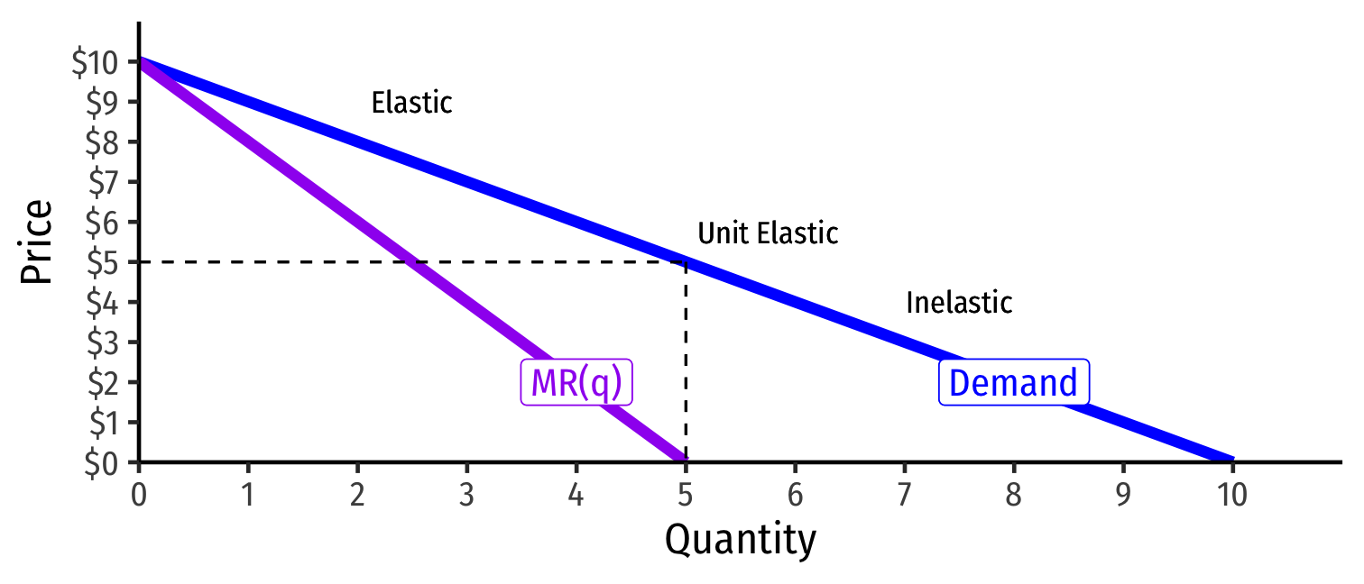
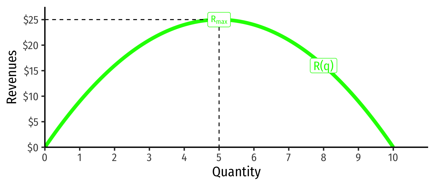
| Demand Price Elasticity | MR(q) | R(q) |
|---|---|---|
| |ϵ|>1 Elastic | Positive | Increasing |
| |ϵ|=1 Unity | 0 | Maximized |
| |ϵ|<1 Inelastic | Negative | Decreasing |
Strong relationship between price elasticity of demand and revenues
Monopolists only produce where demand is elastic, with positive MR(q)!
- See appendix in today’s appendix for a proof
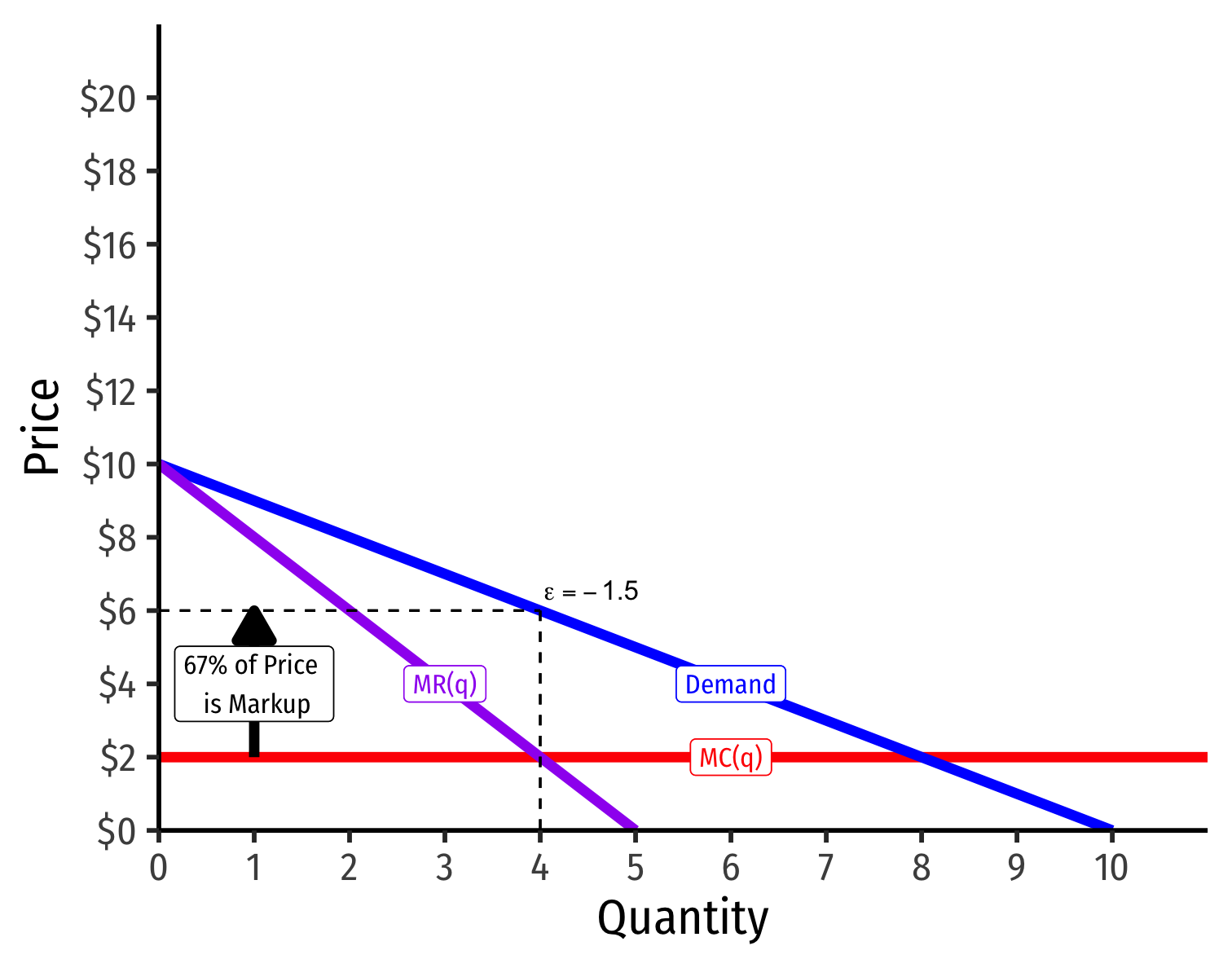
Market Power and Mark Up
Perfect competition: p=MC(q) (allocatively efficient)
Market power defined as firm(s)’ ability to mark up p>MC(q)
- (Even a monopolist’s market power is constrained by market demand!)
Size of markup depends on price elasticity of demand
- ↓ price elasticity: ↑ markup
i.e. the less responsive to prices consumers are, the higher the price the firm can charge

The Lerner Index and Inverse Elasticity Rule I
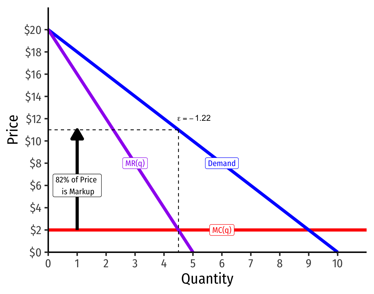
- Lerner Index measures market power as % of firm's price that is markup above MC(q)
L=p−MC(q)p=−1ϵ
- i.e. L×100% of firm’s price is markup
- L=0⟹ perfect competition
- 0% of price is markup, since p=MC(q)
- As L→1⟹ more market power
- 100% of price is markup

See today's appendix for the derivation.
The Lerner Index and Inverse Elasticity Rule II
The more (less) elastic a good, the less (more) the optimal markup: L=p−MC(q)p=−1ϵ
Demand Less Elastic at p∗
Demand More Elastic at p∗
Profit Maximization Rules, Redux
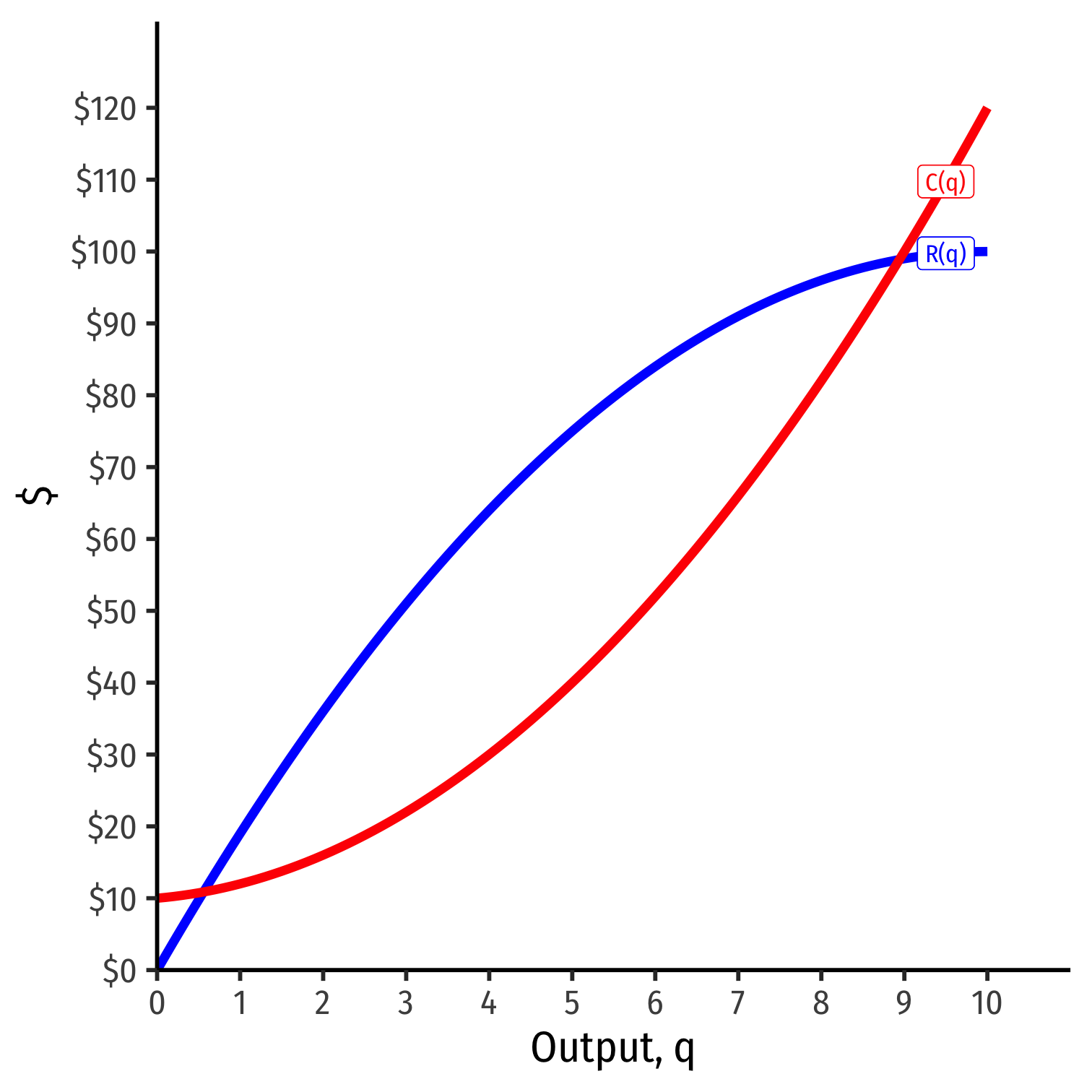
Visualizing Total Profit As R(q)-C(q)
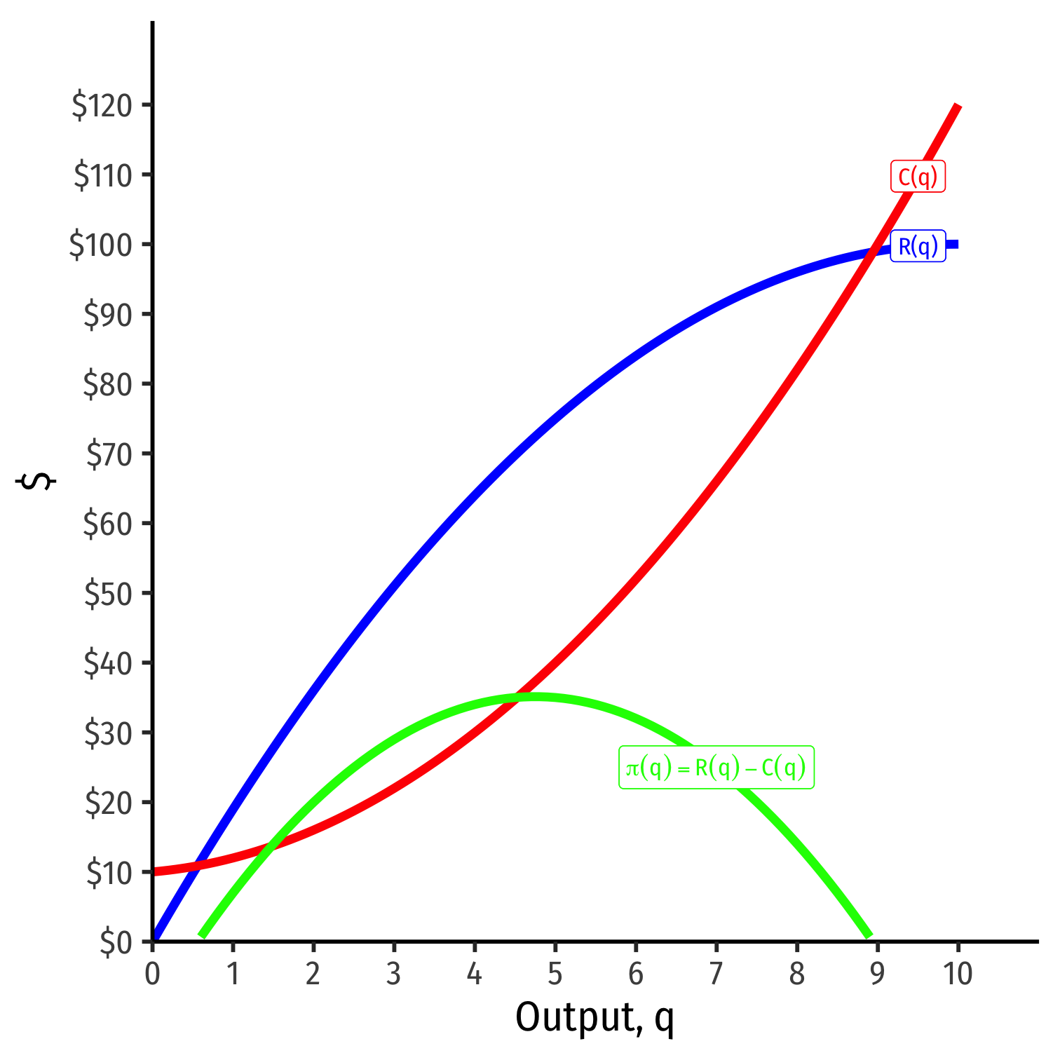
- π(q)=R(q)−C(q)
Visualizing Total Profit As R(q)-C(q)
- π(q)=R(q)−C(q)
Visualizing Total Profit As R(q)-C(q)
π(q)=R(q)−C(q)
Graph: find q∗ to max π⟹q∗ where max distance between R(q) and C(q)

Visualizing Total Profit As R(q)-C(q)
π(q)=R(q)−C(q)
Graph: find q∗ to max π⟹q∗ where max distance between R(q) and C(q)
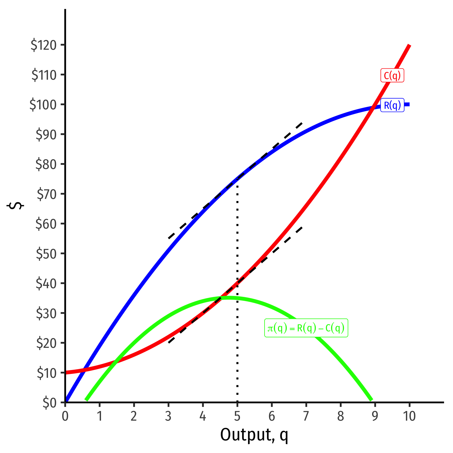
Slopes must be equal: MR(q)=MC(q)
Visualizing Total Profit As R(q)-C(q)
π(q)=R(q)−C(q)
Graph: find q∗ to max π⟹q∗ where max distance between R(q) and C(q)
Slopes must be equal: MR(q)=MC(q)
- At q∗=5:
- R(q)=75
- C(q)=40
- π(q)=35

Visualizing Marginal Profit As MR(q)-MC(q)
At low output q<q∗, can increase π by producing more
MR(q)>MC(q)
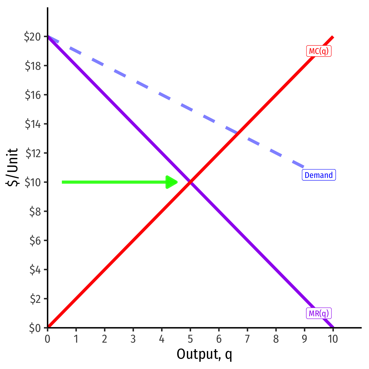
Visualizing Marginal Profit As MR(q)-MC(q)
At high output q>q∗, can increase π by producing less
MR(q)<MC(q)
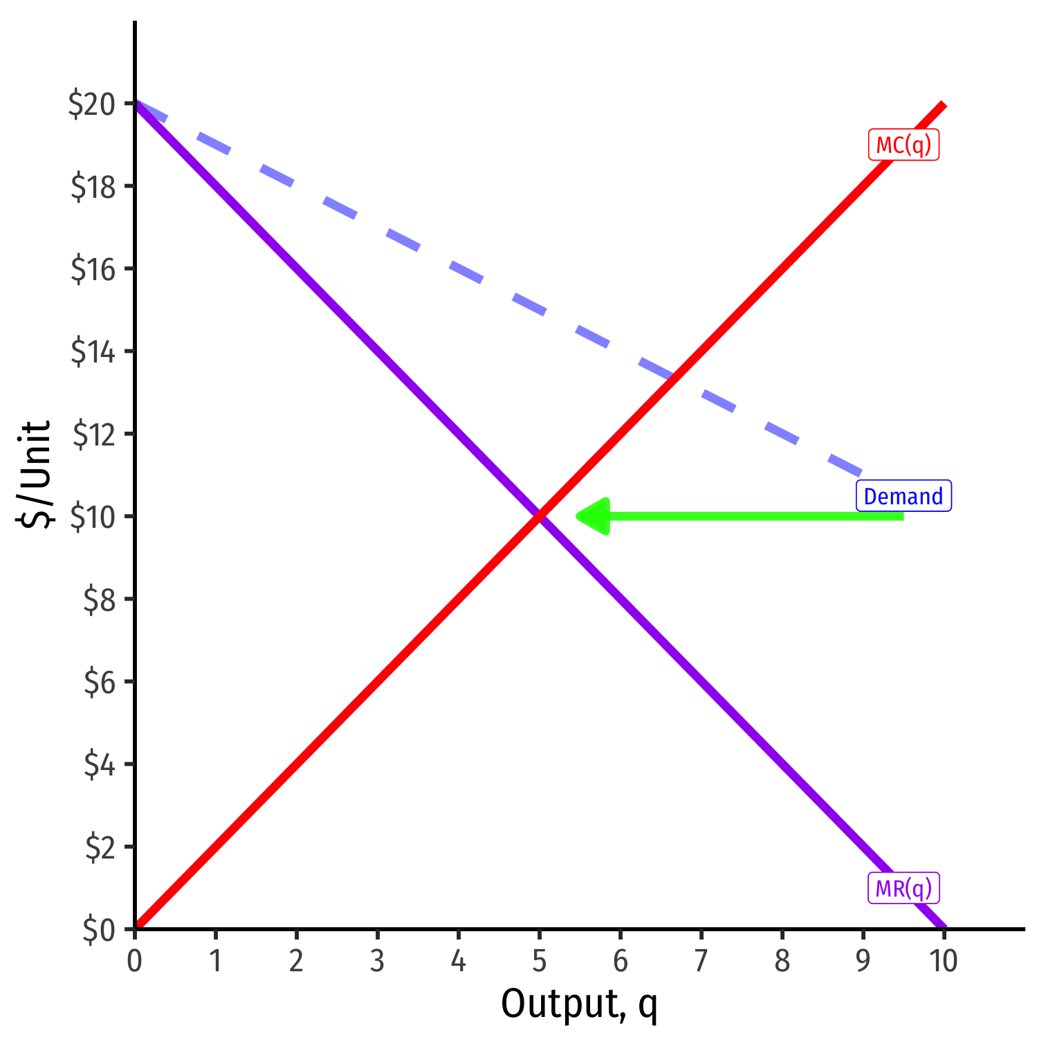
Visualizing Marginal Profit As MR(q)-MC(q)
- π is maximized where MR(q)=MC(q)
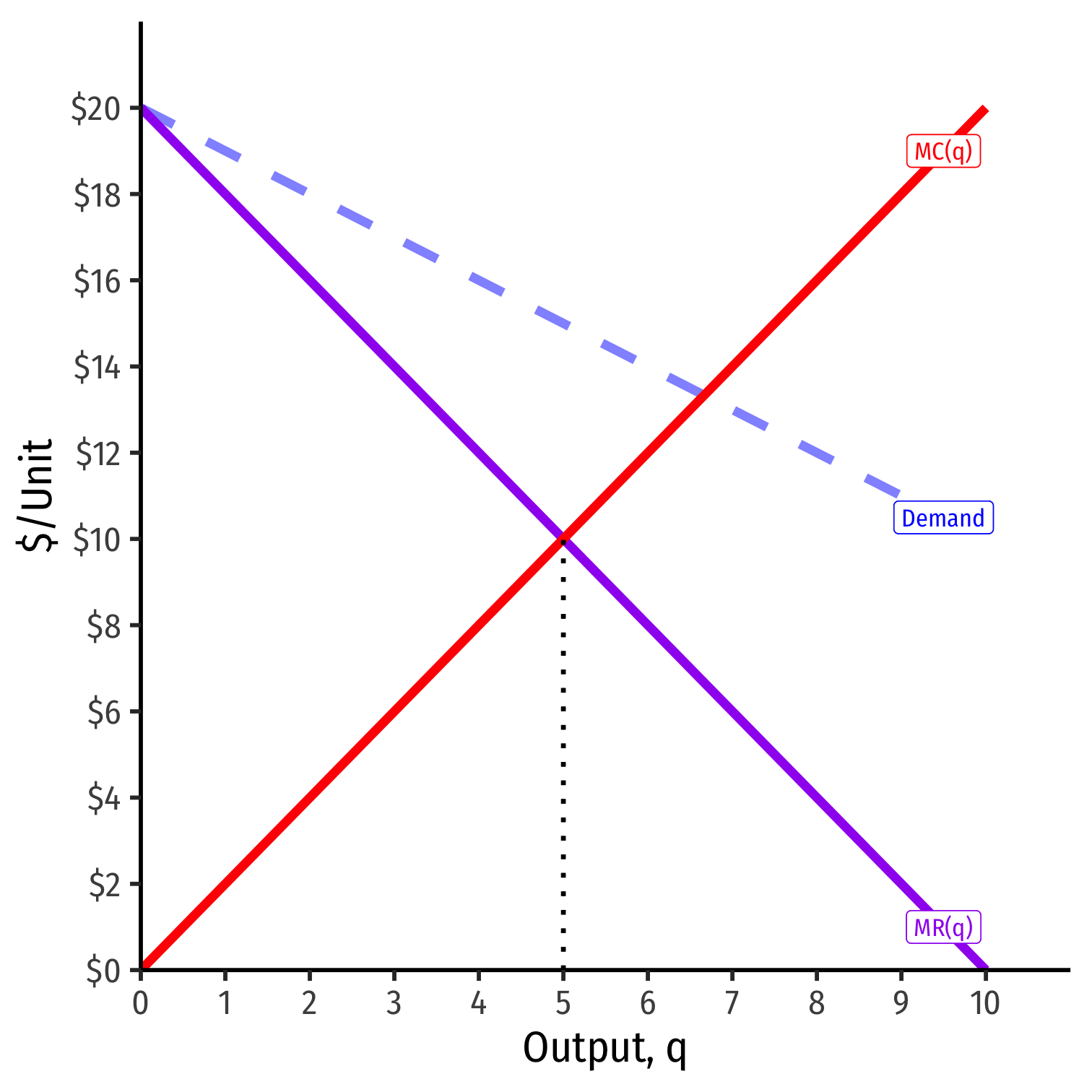
Profit-Maximizing Price and Quantity (Graph)
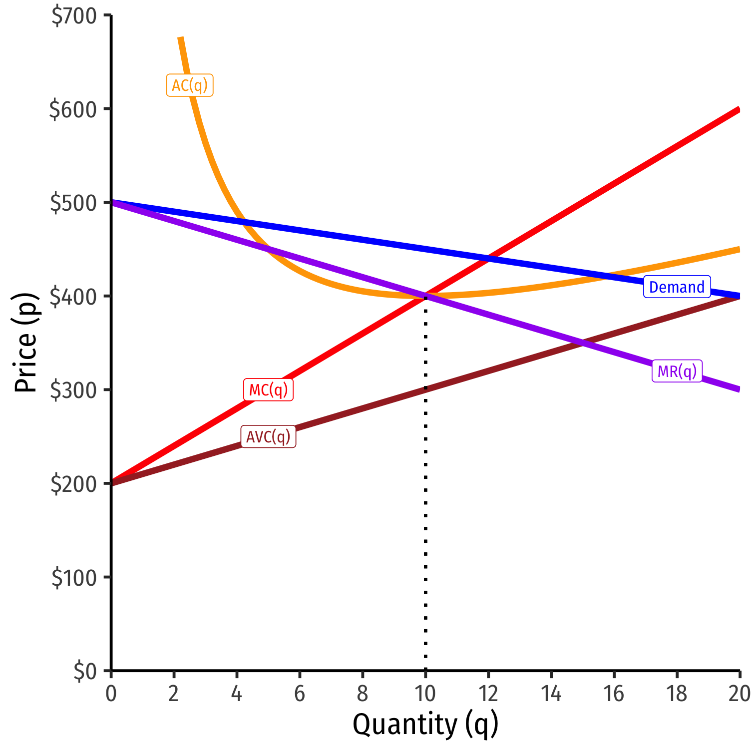
- Profit-maximizing quantity is always q⋆ where MR(q) = MC(q)
Profit-Maximizing Price and Quantity (Graph)
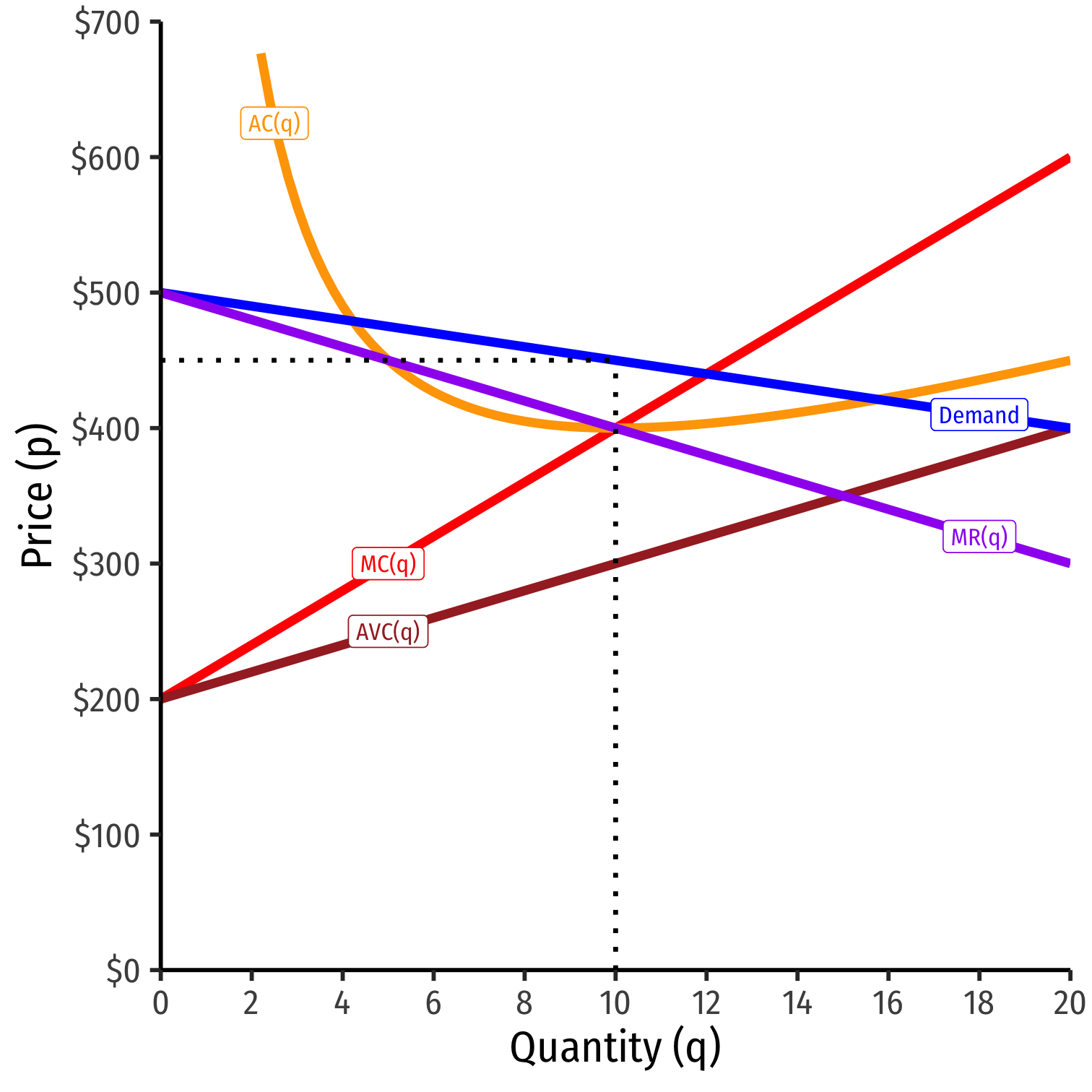
Profit-maximizing quantity is always q⋆ where MR(q) = MC(q)
But monopolist faces entire market demand
- Can charge as high p⋆ as consumers are WTP Market Demand
Profit-Maximizing Price and Quantity (Graph)
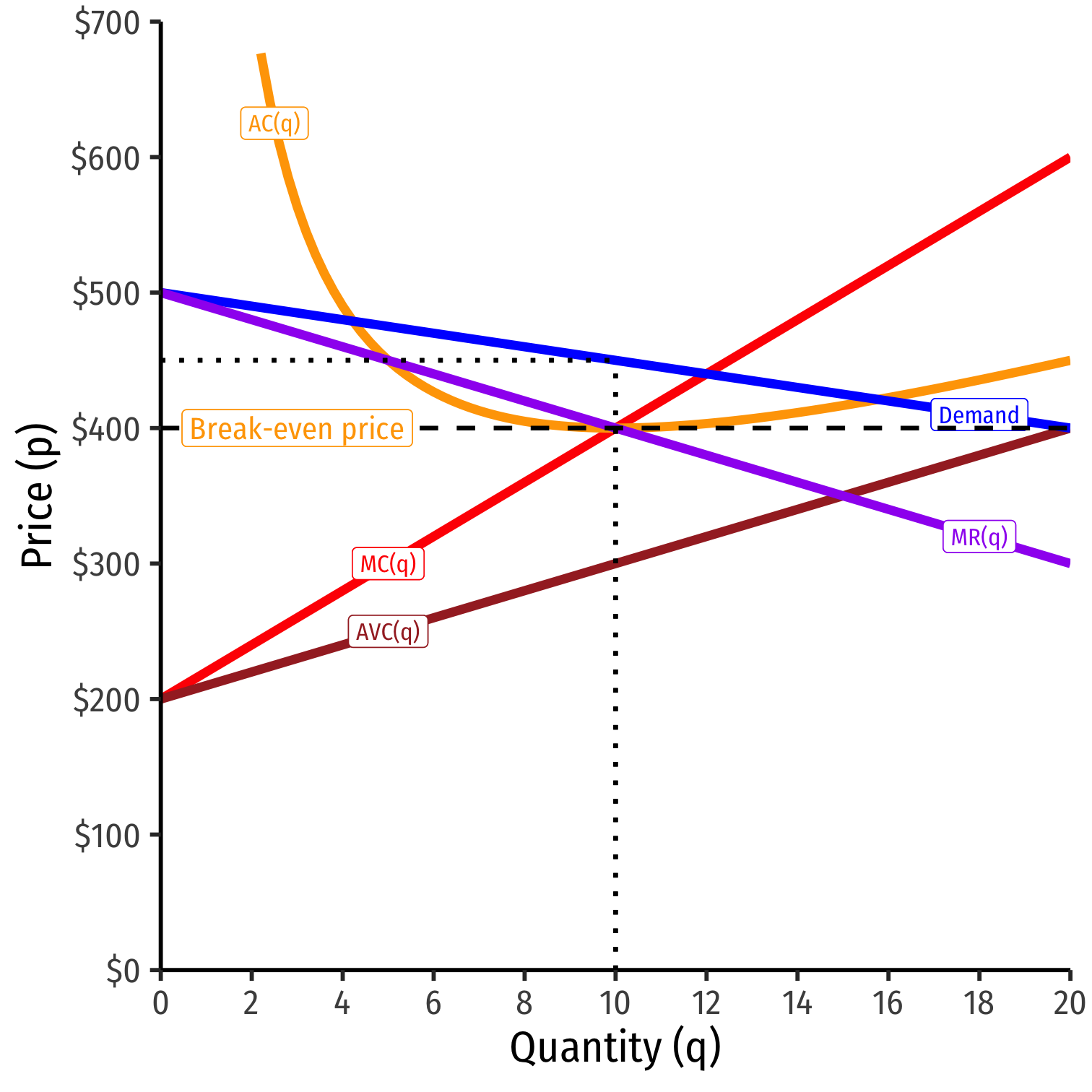
Profit-maximizing quantity is always q⋆ where MR(q) = MC(q)
But monopolist faces entire market demand
- Can charge as high p⋆ as consumers are WTP Market Demand
Break even price p=AC(q)min
Profit-Maximizing Price and Quantity (Graph)

Profit-maximizing quantity is always q⋆ where MR(q) = MC(q)
But monopolist faces entire market demand
- Can charge as high p⋆ as consumers are WTP Market Demand
Break even price p=AC(q)min
Shut-down price p=AVC(q)min
Summing Up Monopolist’s Supply Decisions
- Produce the optimal amount of output q∗ where MR(q)=MC(q)
Summing Up Monopolist’s Supply Decisions
Produce the optimal amount of output q∗ where MR(q)=MC(q)
Raise price to maximum consumers are WTP: p∗=Demand(q∗)
Summing Up Monopolist’s Supply Decisions
Produce the optimal amount of output q∗ where MR(q)=MC(q)
Raise price to maximum consumers are WTP: p∗=Demand(q∗)
Calculate profit with average cost: π=[p−AC(q)]q
Summing Up Monopolist’s Supply Decisions
Produce the optimal amount of output q∗ where MR(q)=MC(q)
Raise price to maximum consumers are WTP: p∗=Demand(q∗)
Calculate profit with average cost: π=[p−AC(q)]q
Shut down in the short run if p<AVC(q)
- Minimum of AVC curve where MC(q)=AVC(q)
Summing Up Monopolist’s Supply Decisions
Produce the optimal amount of output q∗ where MR(q)=MC(q)
Raise price to maximum consumers are WTP: p∗=Demand(q∗)
Calculate profit with average cost: π=[p−AC(q)]q
Shut down in the short run if p<AVC(q)
- Minimum of AVC curve where MC(q)=AVC(q)
Exit in the long run if p<AC(q)
- Minimum of AC curve where MC(q)=AC(q)
The Profit Maximizing Quantity & Price: Example
Example: Consider the market for iPhones. Suppose Apple's costs are:
C(q)=2.5q2+25,000MC(q)=5q
The demand for iPhones is given by (quantity is in millions of iPhones):
q=300−0.2p
- Find Apple's profit-maximizing quantity and price.
- How much total profit does Apple earn?
- How much of Apple's price is markup over (marginal) cost?
- What is the price elasticity of demand at Apple's profit-maximizing output?