2.3 — Cost Minimization — Class Content
Problem Set 3 (on classes 2.1-2.3) is due by 11:59 PM Wednesday March 22 on Blackboard Assignments.
Overview
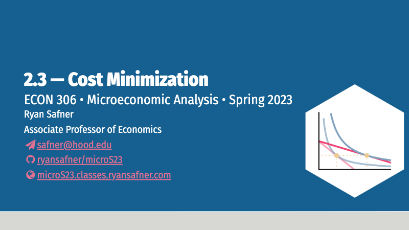
Today we put our tools together (production functions/isoquants and isocost lines) to solve the firm’s cost minimization problem. Again, we do not solve this constrained optimization problem with calculus, but by looking graphically, and using an algebraic rule that should make intuitive sense.
Again, these tools and rules are almost identical to how we solved the consumer’s problem. Compare
Consumers:
- choose goods to maximize utility subject to their budget constraint
- budget constraint (line) is what is fixed
- get on highest indifference curve tangent to budget constraint
Producers (Firms):
- choose inputs to minimize cost subject to producing the optimal amount (their constraint)
- isoquant curve is what is fixed (want to produce a specific amount!)
- get on lowest isocost line tangent to isoquant curve
We finally wrap up with a discussion of returns to scale.
Readings
- Ch. 6.4-6.7 in Goolsbee, Levitt, and Syverson, 2019
Optional/Recommended Reading
- Increasing Returns — my newsletter with the theme of increasing returns
Appendix
See the online appendix for today’s content:
Assignments
Problem Set 3 Due Wednesday March 22
Problem Set 3 (on classes 2.1-2.3) is due by 11:59 PM Wednesday March 22 on Blackboard Assignments.
Slides
Below, you can find the slides in two formats. Clicking the image will bring you to the html version of the slides in a new tab. The lower button will allow you to download a PDF version of the slides.
You can type h to see a special list of viewing options, and type o for an outline view of all the slides.
I suggest printing the slides beforehand and using them to take additional notes in class (not everything is in the slides)!
